Chapter 10 Lubrication Theory
Lubrication theory is used to describe fluid flows in a geometry where the characteristic lengthscale in one dimension is significantly smaller than the others. Lubrication theory is important for understanding lubrication of components in machinery such as a fluid bearing, and in biological fluid dynamics such as understanding the flow of red blood cells in narrow capillaries.
10.1 Lubrication approximation for flow in a thin layer
Let be a characteristic vertical lengthscale and be a characteristic horizontal lengthscale in the direction of fluid flow. In the lubrication approximation we assume the layer is shallow such that
| (10.1) |
In addition, let be the scale of the horizontal velocity (in the direction of fluid flow). From incompressibility () we know that the vertical velocity must scale as . Note, here we are assuming that the flow is two-dimensional with no dependence on the coordinate out of the page (). We will now non-dimensionalise the Navier-Stokes equations using these scales. As a recap here, refer back to chapter §4 on Dimensional Analysis.
We now introduce dimensionless variables (denoted by the tilde)
| (10.2) |
For a Newtonian fluid, the equation for mass balance (see §2.8) becomes
| (10.3) |
owing to the choice of scalings for the the vertical velocity. The horizontal momentum equation (see §2.9) is
| (10.4) |
Dividing by , the equation becomes
| (10.5) |
From this non-dimensional version of the equation we can see that inertia can be neglected if the modified Reynolds number based on and satisfies
| (10.6) |
with timescale . Choosing pressure scale , the horizontal momentum equation can finally be approximated as
| (10.7) |
Using these scales for the pressure and time we can repeat the non-dimensionalisation for the vertical momentum equation:
| (10.8) |
We find that to leading order (setting ) inertia can be neglected and the pressure is independent of vertical coordinate i.e. . Here, we have ignored any body forces such as gravity. If we were to include gravity we’d find the scaling of the vertical momentum equation implies that the pressure is hydrostatic (with and ). We will come across this in some of the examples we cover later.
10.2 Squeeze flow
10.2.1 Thrust bearing
Let’s first consider the squeeze flow in a thrust bearing. Figure 10.3 shows the geometry and coordinate system where the bearing remains stationary and the plane underneath the fluid moves with horizontal velocity . The fluid film wedge generates a hydrodynamic pressure that supports an applied load on the bearing with a small tangential force for good lubrication. We would like to calculate the pressure in the fluid and hence the forces exerted on the bearing by the fluid. To solve the lubrication problem we: describe the geometry, solve for (almost) unidirectional flow, apply mass conservation to close the system, and calculate quantities of interest in this case the forces on the bearing.
Geometry The fluid film thickness is given by the geometry of the bearing
| (10.9) |
For the thin film approximation we require . This means that the gradient of the bearing is also small, , and flow is predominantly in the direction.
Unidirectional flow Given that the flow is approximately in the direction we can write the velocity as . The momentum equations are then
| (10.10) |
The -momentum balance tells us that the pressure is independent of . If is independent of then must also be independent of . Hence, we can integrate the -momentum balance twice:
| (10.11) |
using the boundary conditions and since the underlying plane is moving and the bearing is stationary (and we have assumed no-slip on both surfaces). The final quantity to determine is the pressure gradient .
Mass conservation In order to calculate the pressure (and pressure gradient) we can use global mass conservation and boundary conditions on the pressure. By global mass conservation we know that the volume flux (per unit -width) must be constant. We also assume that away from the bearing the pressure must be atmospheric, at . In more detail:
| (10.12) |
Integrating the pressure and applying the boundary conditions at gives
| (10.13) |
Applying the boundary condition at allows us to determine the constant volume flux :
| (10.14) |
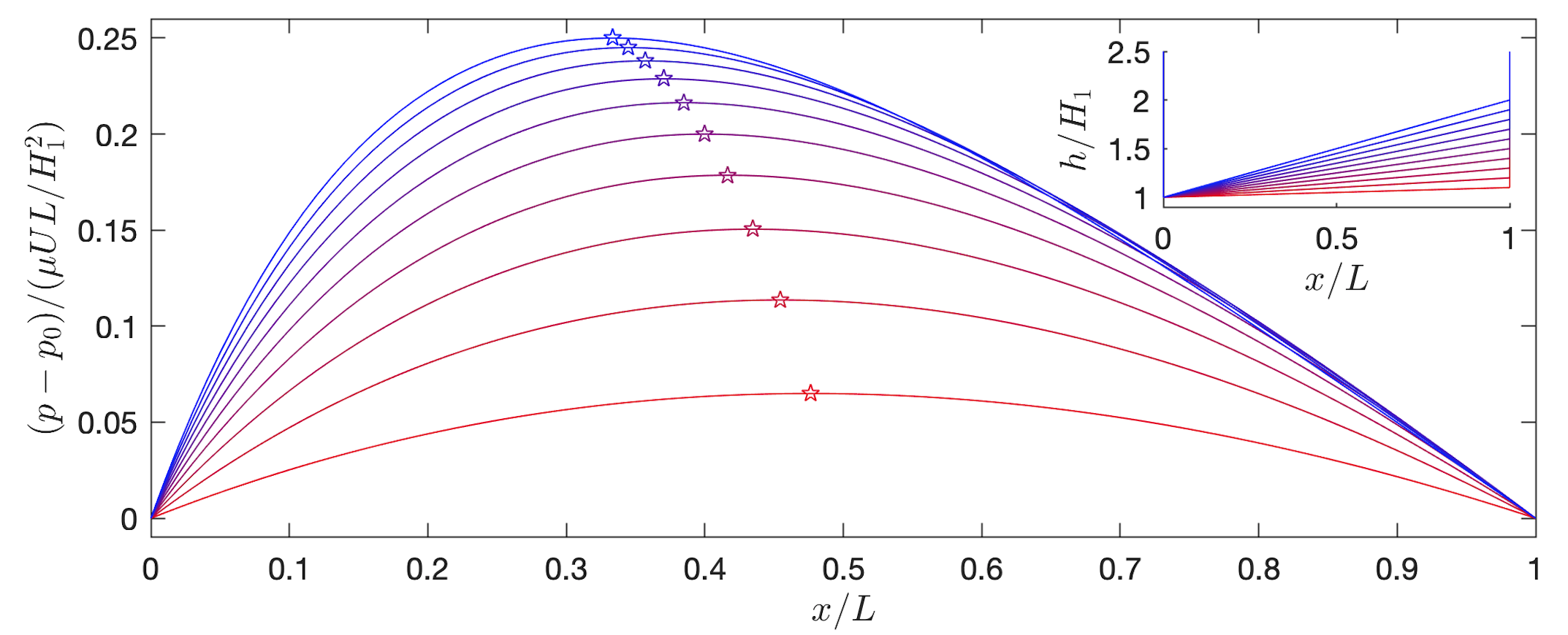
The volume flux and the pressure could then be substituted back into the expression for the horizontal velocity . The pressure gradient generated by the lubrication flow ensures that the mass flow is constant through the narrow gap. From the pressure increases up to a maximum when is zero. The pressure then decreases again to match the atmospheric pressure at .
| (10.15) |
The pressure field is plotted for different angle bearings in figure 10.4. In a similar manner, we could look at what the tangential stress on the boundaries is by calculating at .
Forces A thrust bearing is supposed to support high applied loads with reduced friction. To see when this is the case we can calculate the force on the boundaries per unit -width:
| (10.16) |
where
| (10.20) |
where we have kept only the leading order terms []. The normal vector is
| (10.23) |
Remember, a normal vector to a plane specified is given by . The unit normal vector is then defined as . For the bearing, the boundary is . Hence, the unit normal is given by
| (10.24) |
The normal force (above atmospheric pressure) is
| (10.25) |
Similarly, we can calculate the tangential force:
| (10.26) |
It would be a good exercise to check these! In the thin film limit , the normal force is much larger than the tangential force, and hence this is a low friction bearing.
10.2.2 Cylinder approaching a wall
The second squeeze flow problem we will consider is a cylinder approaching a wall. We will carry out a similar procedure to the previous problem. Figure 10.5 shows the geometry of the problem. A cylinder of radius falls vertically towards a horizontal plane with minimum gap between the cylinder and the plane, where in the thin film limit. There are non-slip boundary conditions on the cylinder and on the plane.
Geometry The height of the fluid underneath the cylinder in the limit of () is
| (10.27) |
This expression for the height gives the horizontal lengthscale in the problem . This lengthscale is much smaller than the radius of the cylinder () so is consistent with the approximation of . This lengthscale is also much larger than the minimum gap () so the flow is in the thin film limit and can be approximated as unidirectional.
Unidirectional flow Following the same method as for the thrust bearing, we can write the unidirectional flow horizontal velocity as
| (10.28) |
Mass conservation The total volume flux (per unit -width) is given by
| (10.29) |
Since the vertical velocity of the cylinder is we know the volume leaving a region per unit time is [where ]. This must be equivalent to the volume flux. Hence, and
| (10.30) |
using the boundary condition and .
Forces As in the case of the thrust bearing, the normal force per unit-z width (above atmospheric pressure) is
| (10.31) |
If the cylinder is sedimenting under gravity we know that constant. Substituting this in we find
| (10.32) |
Hence, the cylinder does not reach the wall in finite time.
10.3 Free surface flow
In the previous two problems we have considered the squeeze flow between two surfaces where the boundary condition on each surface is no-slip (i.e. the velocity parallel, or approximately parallel, to the surface is zero). In this next section, we will consider free surface flows where we remove one surface so the fluid is ‘free’ to move and its location needs to be determined as part of the problem. In particular, we will consider the shape of a drop on a horizontal plane controlled by either capillary or gravitational forces. To understand when these forces are applicable we will first introduce the idea of surface tension.
10.3.1 Surface Tension
Surface tension is a property of a free surface which appears due to the asymmetry of intermolecular forces acting in the interfacial region (typically of nanometric width). As one goes to smaller length scales, surface forces () begin to dominate volume forces (). In particular, the surface tension force typically begins to dominate gravity when the length scale goes below millimetres-cm.
In the general case, for a free surface between a viscous liquid and a second viscous fluid (gas or liquid), if we assume that the velocity is continuous across the interface, there are 4 boundary conditions required for the 4 unknowns (3 velocities, which are not fixed, and 1 variable representing the free surface shape). These are provided by kinematic and dynamic boundary conditions.
Kinematic Boundary Condition Consider a free surface given in implicit form as with corresponding to fluid 1 and corresponding to fluid 2. The free surface moves with the velocity of the fluid, so that fluid particles which begin on the free surface remain there. In other words, the surface ‘follows the fluid’. This means that we have conservation of along the fluid paths of the surface particles, i.e. the material derivative of is zero:
| (10.33) |
E.g. For a two-dimensional flow, suppose the free surface is defined as . Then . At the free surface we have and a unit normal vector which point out of fluid 1. For so that we find that
| (10.34) |
Dynamic Boundary Condition To obtain a dynamic boundary condition, one applies Newton’s II Law to the surface (an interface) separating the two fluids. Because there is no mass to the surface ( and external body forces are negligible), the forces acting on the surface from either side, i.e. caused by the stresses from the two fluids, must balance with any forces that occur from inside the interface.
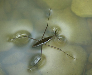
To calculate the forces from inside the interface we will be interested in surface tension. Surface tension acts like an elastic membrane on the surface of a liquid and forces it to attempt to minimise its area (crudely, this is because it is energetically favourable for molecules to be in the bulk of the liquid, rather than at its surface). This force is responsible for a whole host of effects ranging from the suspension of small objects (e.g. water striders) through to the breakup of liquid jets (e.g. from a tap in a kitchen), which occurs when the liquid can reduce its surface area by forming a series of spheres (drops) rather than one cylinder (the jet), see figure 10.6. Problems involving surface tension are known as capillary flows.
The surface tension force (taken to be constant here), per unit length of line, is directed tangentially along the surface which is parameterised by coordinates with tangent vectors in these directions . Our control volume will have ‘lower edge’ at and now has a surface tension force tugging at all four ends in the tangential direction.
Consider a control volume of length and width along the interface equal to whose height is negligible compared to , see figure 10.7. This gives a force balance of
at . Dividing through by and taking the limit we find that
| (10.35) |
where we have defined the curvature of the interface using
| (10.36) |
To arrive at this expression we know that and . Differentiating with respect to interface coordinates gives
| (10.37) |
| (10.38) |
This can be simplified further by noting that . Hence, the curvature can be written as
| (10.39) |
10.3.2 Bond number
We have seen from equation (10.35) that the stresses tangential to the interface are continuous, whereas the normal stress has a jump caused by the surface tension force . Hence, the pressure generated by surface tension is of the order , where is a characteristic lengthscale in the problem which is approximately the radius of curvature of our interface. Therefore, capillary forces will be important when this is comparable to the pressure generated by gravitational forces, i.e. the hydrostatic pressure which occurs when
| (10.40) |
where is known as the capillary length and is the Bond number. For water in air, where N/m, we have mm. Therefore, for large scale flows, such as sea waves, surface tension has no effect, but for small scale flows, such as those encountered in micro and nanofluidics, its importance far outweighs that of gravity.
10.3.3 Capillary number
In many cases, we are interested in knowing the shape of a liquid drop or bubble whose flow has negligible force in comparison to the surface tension forces. In the latter case, for low Reynolds number flows, where viscous forces dominate inertial ones, looking at the dynamic boundary condition we can see that the viscous force has magnitude whilst the surface tension force is . The ratio of these forces gives the capillary number:
| (10.41) |
and when the flow within the drop has a negligible effect on the free surface, so that the shape can be calculated independently of the flow (a huge simplification).
10.3.4 Capillary drop
Let’s consider a liquid drop sat on a horizontal surface. For simplicity, let’s consider a two-dimensional drop pinned at where , see figure 10.8. In the limit of small capillary number , we can neglect the stress in the drop and calculate the shape of the drop from the dynamic boundary condition:
| (10.42) |
This is known as the Young-Laplace equation. We can parametrise the free surface in terms of a height function , so that , see figure 10.8. Then
| (10.43) |
From our -momentum equation we find the pressure in the fluid is hydrostatic . We assume the ambient fluid has a uniform pressure . Substituting these into the dynamic boundary condition (10.42) gives
| (10.44) |
where is the (constant) pressure drop across the interface. Hence,
| (10.45) |
This is a second order PDE for and hence we must specify a boundary condition on or its derivative at each end of the free surface. On top of this one either needs to specify the pressure drop or, more often, the volume of the liquid which can then be used to find .
In the lubrication limit for small bond numbers , this reduces to
| (10.46) |
with solution a parabola
| (10.47) |
where we have the used the pinned boundary condition . We see that for meaningful solutions we need as represents the pressure in the gas minus the pressure in the liquid (which we expect to be higher for a drop, due to surface tension). If we calculate the volume of the drop we can see how the pressure and volume of the drop are related:
| (10.48) |
In this solution we assumed the drop was pinned at points . This is known as a pinned contact line. An alternative boundary condition would be to prescribe the contact angle , the angle at which the free surface meets the horizontal plane, see figure 10.8. This then gives a boundary condition on the gradient at . In this case the position of the contact line would be found as part of the solution.
The prescribed contact angle will depend on the liquid-solid-gas combination in question: if the solid is ‘wettable’ (aka hydrophilic for water) this angle will be small (i.e. close to zero), so the drop spreads out a lot (e.g. water on glass), whereas if the angle is high (close to ) then the solid is non-wettable (aka hydrophobic) and the drop beads up (e.g. water on a lotus leaf).
10.3.5 Gravitational spreading
When the lengthscale of the liquid drop becomes large, gravitational forces begin to dominate over capillary forces (large Bond number) and viscous forces begin to dominate over surface tension (large capillary number). We can therefore neglect the jump in the normal stress at the free surface but now need to calculate the flow within the fluid. Let’s consider the shape of an axisymmetric drop on a horizontal surface under the influence of gravity, or equivalently, let’s consider the axisymmetric, gravitational spreading of a thin film layer on a horizontal surface, see figure 10.9.
Geometry Unlike the squeeze flow problems, the geometry is unknown and will be determined as part of the solution. In addition, we are now in a cylindrical polar coordinate system. We write the surface of the thin-film as
| (10.49) |
where is the vertical coordinate, and in the radial coordinate parallel to the horizontal plane.
Unidirectional flow In the thin film limit so the flow is predominantly in the direction. We can write the velocity as . The - and -momentum equations are then
| (10.50) |
[Note, here we have taken the lubrication approximation of the Stokes equations written in cylindrical polar coordinates. In this case, the two-dimensional version is the same if we replace and .] We have also now introduced body force . Integrating the -momentum equation and applying boundary condition gives
| (10.51) |
Hence, the pressure in the fluid film is hydrostatic. Substituting this into the -momentum equation we have
| (10.52) |
The right-hand side is independent of so the flow is driven by the slope of the free-surface. The boundary conditions on the no-slip underlying plane and the free surface are:
| (10.53) |
The second condition here is the dynamic boundary condition. Because we are considering large capillary numbers there is no jump in stress at the boundary (and the ambient fluid is assumed to have a negligible viscosity). Hence, we find the shear stress must be zero at the free surface.
Finally, integrating the momentum equation and applying the boundary conditions gives radial velocity profile
| (10.54) |
Mass conservation For mass conservation we consider a cylindrical annulus from , see figure 10.10. The volume of fluid entering the annulus at radius per unit time is , where is the radial volume flux. Similarly, the volume of fluid leaving the annulus at radius is . In addition, because the top surface is able to move volume can also leave the annulus vertically at a rate per unit time of . Here, I have used kinematic boundary condition , which is valid when . Equating these volumes to ensure volume conservation gives
| (10.55) |
[Note, the is present because we need to think about the volume flux in to and out of the entire annulus. If we were in a two-dimensional geometry, we could ignore this factor and then replace .] As before, we can calculate the volume flux by considering the flux out of a cylinder of radius :
| (10.56) |
where we have used surface element in a surface of constant radius . Substituting this flux into the mass conservation equation gives
| (10.57) |
We now need to solve this Partial Differential Equation (PDE) for the free boundary . As an aside, let’s integrate the PDE in between and the boundary where (it’ll be clear why in a moment):
| (10.58) | ||||
| (10.59) |
The second term on the left-hand side is zero because the film has zero height at the edge, . The right-hand side is zero because the flux at the centre and the edge is zero, . Therefore, the volume of the drop is constant:
| (10.60) |
where we have used volume element in cylindrical polar coordinates. If instead, we were able to introduce fluid at the centre of the flow with some non-zero volume flux we would have condition as and .
Solving for the free boundary
We would like to solve the following PDE (non-linear diffusion equation) subject to the global constraint that the volume is constant:
| (10.61) |
Scaling the equation of motion and global mass conservation using characteristic height, radial and time scales and gives
| (10.62) |
which can be rearranged to
| (10.63) |
Since there are no more scales in the problem (assuming the initial condition was a sufficiently long ago to be irrelevant) it suggests we such look for a similarity solution of the form
| (10.64) |
with the edge of the film at . These solutions are self-similar which means that by appropriately scaling the radius and height of the film by a power of the time evolution of the current falls onto a universal curve (we’ll plot the solution up later to show this more clearly). Let’s substitute this ansatz into the PDE and constraints. With some algebra with arrive at:
| (10.65) |
where the prime denotes differentiation w.r.t . The power of this type of solution is that we’ve turned a PDE into an ODE for which is significantly easier to solve. We can now make progress with the ODE as follows:
| (10.66) | ||||
| (10.67) | ||||
| (10.68) |
since we want . Integrating again we get
| (10.69) |
Finally, applying our volume constraint we can determine and hence solution
| (10.70) |
or equivalently
| (10.71) |
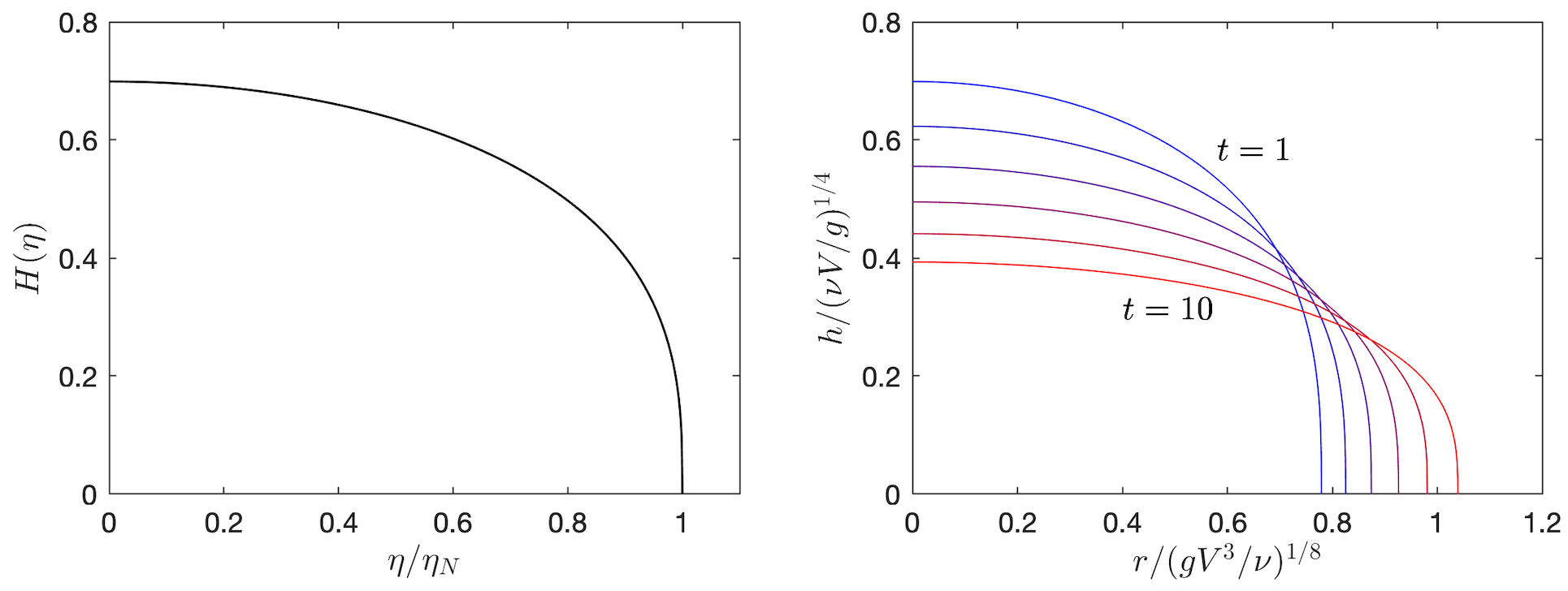
Figure 10.11 plots the solution to demonstrate the self-similar behaviour.
Shape of the nose
To investigate the shape of the nose we let . Substituting into the governing equation when gives
| (10.72) | ||||
| (10.73) |
Matching the powers of gives . The shape of the nose is then . The gradient is therefore singular at the nose, but not too singular that the flux boundary condition is still satisfied.
10.3.6 Gravitational spreading down an inclined plane
Let’s now consider the shape of a two-dimensional drop spreading down an inclined plane of slope . is the downslope coordinate and is the vertical coordinate perpendicular to the slope. The body force is then . The fluid is released from a fixed point such that and the ambient has constant pressure .
The Lubrication approximation is then
| (10.74) |
Integrating the y-momentum equation gives hydrostatic pressure . Calculating the velocity field, integrating across the depth to get the volume flux, and applying mass conservation, we arrive at evolution equation
| (10.75) |
A similarity solution does not exist for the full governing equation. Instead we will consider one particular limit.
Problem: Let’s consider a constant volume release (per cross-slope distance) of viscous fluid at such that . After a long time the nose (or front) of the current has travelled a distance . We want to find a similarity solution for . The volume constraint can be written as
| (10.76) |
Scaling the evolution equation to look for the dominant terms gives
| (10.77) | |||
| (10.78) | |||
| (10.79) |
Looking at the relative size of the terms, for , we can neglect the RHS of the evolution equation. The system we want to solve is then
| (10.80) |
Scaling the remainder of the equations suggest the following scales for the vertical and horizontal coordinates
| (10.81) |
Given these scales we will look for a similarity solution of the form
| (10.82) |
The governing equations then become
| (10.83) |
Integrating gives we can then determine the nose position
| (10.84) |
The similarity solution is then
| (10.85) |
We can see from the similarity solution that the thickness is finite at the front . This is because we have neglected a term in the evolution equation which becomes important when you are near the front. To find the shape of the front (how this jump in the thickness is rounded off) we can substitute in into the evolution equation. This gives two possible values for (assuming the neglected term is one of the scales). We know we need to match onto the finite thickness height so must have a cube-root singularity at the nose. This just says that at the nose, the first term on the LHS and the term on the RHS dominate. Alternatively, we could pose ansatz where has some unknown functional form to be determined and is the thickness at the front and solve for using the full equation.