Chapter 2 Mathematical Modelling of Fluid Flow
In this chapter, we will derive the mathematical model governing the motion of fluids. In summary, these will be the Navier-Stokes equations, but on the way we will encounter the Eulerian and the Lagrangian descriptions of fluid motion, the deformation of infinitesimal fluid particles, Cauchy’s notion of stress and his equation for motion of continuum, Euler’s equations for motion of an ideal fluid, etc. We begin with the definition of a fluid.
2.1 Definition of a fluid
Definition
Fluid: A continuum substance that cannot withstand shear stress without continually deforming.
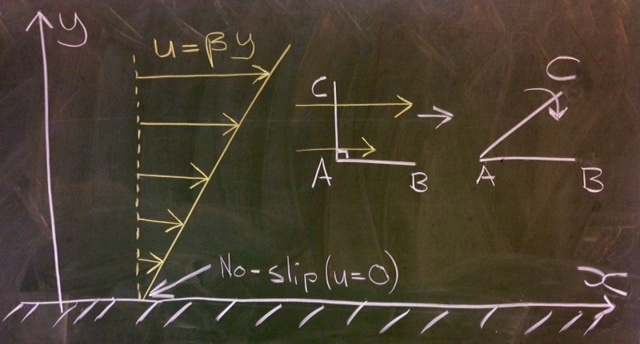
Consider a thin layer of material sandwiched between two plane walls, as shown in Figure 2.1. Under the action of the applied traction, , each layer of the material slides proportional to the distance from the lower wall, which is held fixed. The displacement is given by . The shear in this scenario is . At long times, approaches a constant for a solid. But for a fluid, keeps increasing at a constant rate, i.e., , where is the rate of shear.
There are other definitions of a fluid that, while appropriate to be used at more elementary treatments of fluid dynamics, are inadequate for the purposes of deriving mathematical models for describing their behaviour. One such definition is that a fluid is a substance that assumes the shape of its container. This definition is inadequate for our purpose because there is no mention of gravity, the driving force that makes some of those substances, namely liquids, conform to the shapes of their containers. But even for gases, this definition does not furnish the defining element instrumental in deriving the governing equations for fluid flow – the internal stress experienced by elements of the fluid and the resulting deformation.
While our definition addresses some of the shortcomings of the more elementary definitions, it has left some terms undefined. For instance, what is a continuum substance? What is a shear stress? How does one quantify continual deformation? Also note that the definition does not constrain the magnitudes of the shear stress or that of the deformation, nor does it specify any relation between the two.
Based on this guiding definition, we derive mathematical representations of the laws of conservation of mass, momentum and angular momentum in §2.8, §2.9 and §2.10, respectively. The concepts of deformation rate and stress will emerge in the process. A fluid is any substance that obeys the assumptions that go into the derivations of these mathematical representations. On the one hand, such an exercise rigorously constrains the materials to which the governing equations could be applied. And on the other hand it broadens the scope to include materials that are not commonly classified as fluids but whose mechanics are governed by the equations we derive because they satisfy the underlying assumptions. Understanding the significance of the assumptions that form the basis of the derviation of the governing equations is the objective of this chapter.
2.2 Fluids in Continuum Mechanics
Matter on earth is made up of atoms and molecules, each obeying classical or quantum laws of physics. When dealing with a large collection of molecules, the granularity of molecular composition somehow is lost and/or becomes irrelevant. Properties of matter can then be considered to vary smoothly with location within the material. The emergence of thermodynamics is an example of this. Similarly, when describing motion of macroscopic matter on length scales much larger than molecular scales, it becomes possible to consider the material as a infinitely divisible continuum. The theory of mechanics that arises out of such a consideration is called continuum mechanics.
The continuum approach is accurate when the mean free path , which is the length a molecule of the medium travels between collisions with other molecules, is much smaller than the dimensions of the flow , so that (the continuum limit takes ). Note that is a ‘dimensionless number or parameter’, whose value does not depend on the system of units used. When or , microscopic methods (molecular dynamics for liquids and kinetic theory for gases) are required.
It is worthwhile to ponder briefly about cases where continuum hypothesis fails. Here are two situations:
-
1.
Flow of water through a carbon nanotube: Nanotubes are modern materials consisting of a tube of diameter as small as 0.4 nm. Figure 2.2 shows the use of nanotubes made out of carbon for desalinating water. The basic idea is that while water can flow through the tube, the impurities do not. In this case, the water near the centre of the tube flows faster compared to that near the tube walls, where friction impedes the flow. Thus, the water speed changes over a distance compared to the diameter of the tube, so nm. The molecular mean-free path is about 0.25 nm. In this case, , which is not small. Therefore, the continuum hypothesis is likely to fail.
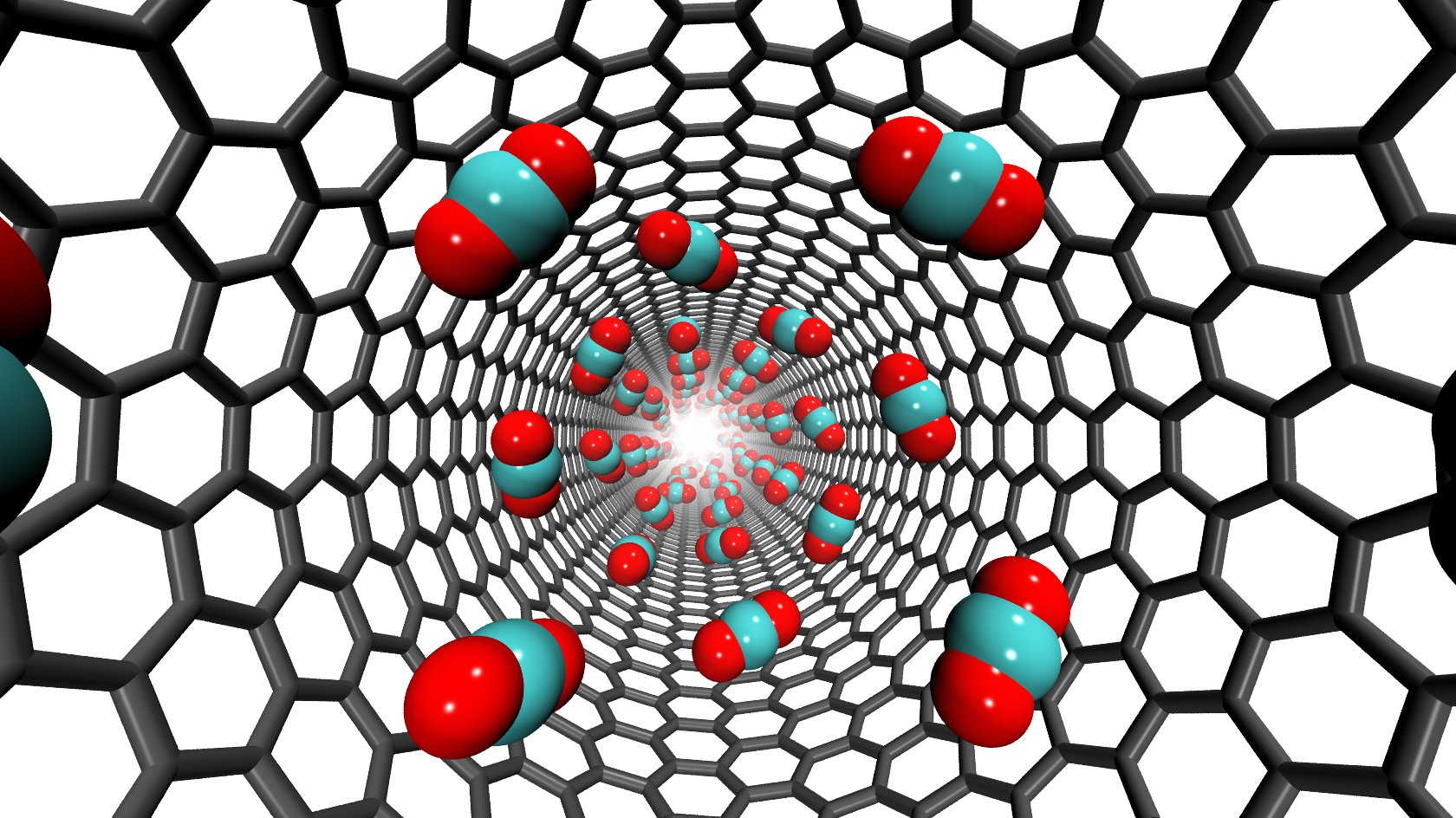
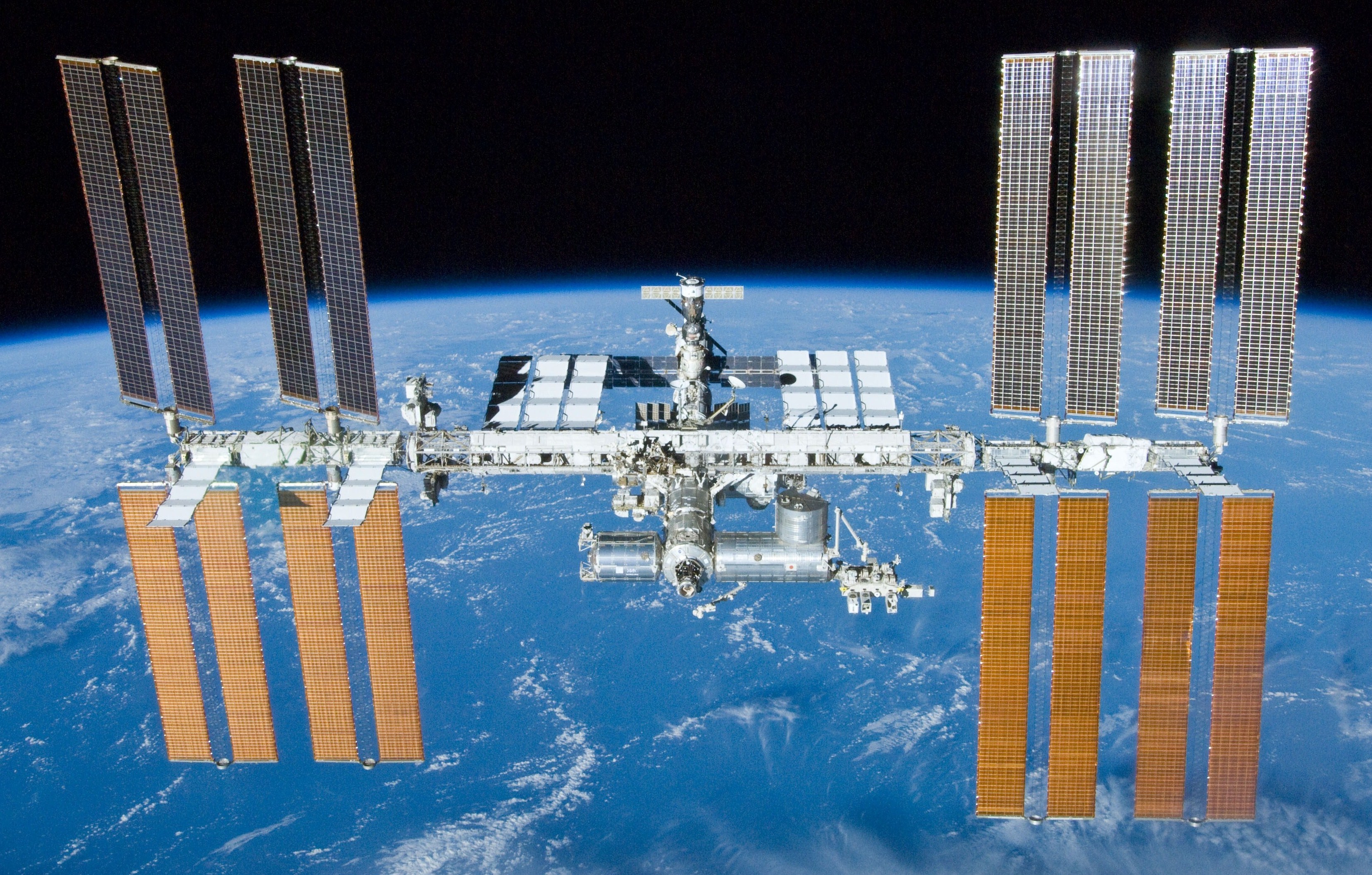
Figure 2.2: Left: An example where continuum mechanics is unlikely to work - a molecular dynamics simulation of a desalination membrane, where water molecules flow through a carbon nanotube (see www.micronanoflows.ac.uk. Right: The International Space Station (source: www.wikipedia.org/wiki/International_Space_Station. -
2.
Motion of the International Space Station (ISS): The ISS is about 79 m 109 m, say approximately m across and orbits the earth at an altitude of 400 km. The atmosphere there is so rarified that the mean free path of gas molecules is km. The ratio is clearly not small, so the surrounding gas cannot be treated as a continuum.
In summary, the continuum approximation of the fluid may fail because (i) the length-scale over which the flow varies is too small, or (ii) the mean free path of the fluid molecules is too large. Both these cases are adequately encapsulated by the ratio .
In day-to-day situation, e.g. flow of water through ordinary pipes, continuum approximation does apply. In that case, every point in space is assigned physical properties such as density, pressure, velocity, stress, etc. Continuous functions of space and time, called fields, are used to represent these physical variables.
2.3 Material properties of fluids
There are five main properties that will be important for us in this module.
-
1.
Density (): The mass of the fluid per unit volume. Air has a density of about 1.2 kg/m and water of 1000 kg/m. Physically, the density of a fluid is determined by its thermodynamic state, and could thus change with pressure and temperature, for instance. If the conditions are such that the density of the fluid does not change appreciably in the flow then such a flow is termed “incompressible”. Under ordinary circumstances, flows of air and water are incompressible. For flow of air around a jet plane, the flow is compressible. And it is certainly so for flow around a supersonic plane.
-
2.
Pressure (): The force a fluid exerts on a wall per unit area. At sea level, air exerts a pressure of about N/m. In SI system, N/m = Pa, a Pascal. Other common units of pressure, especially in atmospheric sciences, are the bar, 1 bar = Pa, and the atmosphere, 1 atm = 101325 Pa. Pressure is also measured in terms of a height of a fluid column, where the fluid is commonly but not necessarily either water or mercury. Normal human blood pressure is purported to range from 80 to 120 mm of mercury.
-
3.
Dynamic Viscosity (): Also known as Newtonian viscosity. It represents the resistance of a fluid to shear. The viscosity is the ratio of the traction applied to the shear rate generated in steady state. In the terminology used in Figure 2.1, . Dynamic viscosity has the SI units of Ns/m or, equivalently, Pa s. An “ideal” fluid or an “inviscid” fluid is one with zero viscosity.
-
4.
Kinematic viscosity (): The kinematic viscosity is the dynamic viscosity divided by fluid density, i.e. . In the SI system, it has units of m/s (note the absence of kg in the units, hence the epithet kinematic).
-
5.
Surface tension (): The surface of a liquid behaves like a stretched membrane. The tension in this “membrane”, measured as force per unit length, is called surface tension. Surface tension has SI units of N/m.
The conditions termed as incompressible and inviscid or ideal are idealizations of real conditions. They are never exactly realized.
2.4 Lagrangian and Eulerian Descriptions
Watch the video on ‘Lagrangian and Eulerian descriptions of fluid flow’ narrated by Prof. John Lumley of Cornell University from the National Committee for Fluid Mechanics. YouTube link: www.youtube.com/watch?v=mdN8OOkx2ko, duration: 27 mins.
The objective in developing the continuum theory of fluids is to decompose the fluid into an infinite number of infinitesimal fluid elements and impose Newton’s laws of motion on each one of them. To do so, it is necessary to label each infinitesimal element of a fluid. There are two common approaches historically employed for doing so. These approaches are called the Eulerian and the Lagrangian descriptions of fluid flow.
2.4.1 Lagrangian description
The Lagrangian description seeks to label and track infinitesimal material volumes of fluid. Their boundaries move with the average speed of the molecules composing the boundaries (only possible in the continuum limit, when there are a large number of molecules on the boundary). Consequently, these volumes always contains the same amount of mass within them. Intrinsic11 1 Here intrinsic quantities are those which do not depend on the total amount of material in the volume. Examples of intrinsic quantities are pressure, temperature, density, as opposed to extrinsic quantities such as mass, volume, etc, which are proportional to the mass of material in the volume. material properties are attributed to the volume by virtue of the material contained in the volume. For example, the velocity, the acceleration, the density, the temperature, the pressure, the concentration of any dissolved species could be attributed to the material volumes. These infinitesimal fluid volumes are also called (Lagrangian) fluid particles or fluid parcels.
A convenient label is the position of an infinitesimal fluid volume, , at some reference time . In the Lagrangian description, the fluid velocity is then given by the fields . This expression stands for the velocity of the Lagrangian fluid particle at time , which was at position at time . Similar interpretation is applied to the density , acceleration , pressure , etc. As an informal convention, we will used capital letters to denote Lagrangian fields.
Caution: It is a common misunderstanding that the fluid inside the material volume is composed of the same material throughout the flow. This is not true. Instead, the correct statement, as mentioned earlier, is that the fluid inside the volume always contains the same amount of mass. Molecules composing the fluid move in and out of the volume such that no net mass leaves or enters the volume.
2.4.2 Eulerian description
The Eulerian description seeks to label the fluid particles by their current location in space. A convenient and common label are the coordinates of the points in space. All physical properties of the fluid are then described as fields over these labels, i.e., the Cartesian coordinates, . For example, the velocity of the fluid is described as a field , which is interpreted as the velocity of the Lagrangian fluid particle that is at location at time . Note that even in the Eulerian description, physical quantities are attributed to the fluid elements and not to the space. Similarly, the density is denoted , the pressure as , the acceleration as , the stress as , etc.
Definition: A Steady Eulerian Field
A steady field is one for which . One of the advantages of the Eulerian description of fluid flow is that in many cases and in properly chosen reference frames, the resulting fields of velocity and pressure are steady. This significantly simplifies the analysis of such flows.
2.4.3 Eulerian versus Lagrangian descriptions
The two descriptions are invoked in fluid dynamics because they simplify different stages of the analysis. Newton’s laws of motion are formulated in the Lagrangian description. Later, we will write the acceleration of Lagrangian particles in terms of the forces they experience. In this formulation, we will need to represent the force exerted by the neighbouring fluid particle as it pushes against the one under consideration, or slides past it. This will require us to track the neighbouring fluid particles as well. Now, the nature of fluid flows is such that the Lagrangian fluid volumes deform significantly with time and so do their neighbours, see Figure 2.3.
The Eulerian description does not suffer from the deformation of volumes. The volume remains fixed because we have defined it to be so. Neighbouring particles also remain in place without deforming. However, the laws of mechanics have been formulated in Lagrangian description. Whilst in the Eulerian description one sits at a fixed position and watches the flow pass (like standing at the bank of a river), in the Lagrangian description we ‘follow the fluid’ (as in a boat flowing with the river or on a weather balloon).
To bridge this gap, we use an Eulerian-Lagrangian map. The most basic element of the map is the transformation between the labels. Given the Eulerian labels and the Eulerian velocity field , the position of Lagrangian fluid particles labeled may be determined by solving for
| (2.1) |
with . In other words, the rate of change of position of a Lagrangian fluid particle is simply the Eulerian velocity at the current location of the fluid particle.
2.4.4 The Material Derivative and Acceleration
There is a section on ‘Material Derivative applied to the concentration of a pollutant in a river’ starting at 12:00 mins in the video on ‘Lagrangian and Eulerian descriptions of fluid flow’ by Prof. John Lumley of Cornell University from the National Committee for Fluid Mechanics. YouTube link: www.youtube.com/watch?v=mdN8OOkx2ko, starting 12:00 mins to the end.
We now use this relation to develop the most common Eulerian to Lagrangian conversion of an operation, differentiation with time. For a generic intrinsic fluid property of arbitrary tensorial rank, the partial derivative with time merely represents the rate of change of at the Eulerian location . It does not account for the fact that at an infinitesimally later time, a different fluid particle now occupies the location . Since most physical laws are formulated in terms of the properties of the Lagrangian fluid particle, it is useful to instead derive an expression for the rate of change of following the fluid particle.
To do so, note that is the property evaluated at the position of the Lagrangian particle labelled by 22 2 Here we mix index notation for with vector notation for .. The location of the particle itself changes with time. Therefore, the rate of change of following the fluid particle is
| (2.2) |
Definition: The Material Derivative a.k.a. The Lagrangian Derivative a.k.a. The Total Derivative a.k.a. The Substantial Derivative
The material derivative is the rate of change of an intrinsic property of a Lagrangian fluid particle expressed in terms of Eulerian quantities. It is symbolically denoted as and is given by the expression
| (2.3) |
Interpretation of the terms in the Material derivative:
-
1.
The first term is the local rate of change at a fixed Eulerian position due to temporal changes.
-
2.
The second is the ‘convective rate of change’ caused by the velocity driving fluid elements through spatial gradients in the quantity of interest. The next example illustrates how a steady (i.e. time independent) Eulerian field could imply a non-zero time-rate-of-change for Lagrangian properties because of the convective rate-of-change term.
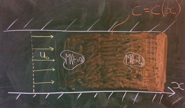
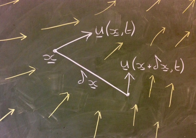
Example: If there is a concentration of pollutant in a river that flows steadily with constant speed (see Figure 2.4), how does the concentration change in a fluid element that ‘follows the fluid’?
Note that (a) the concentration at a fixed point does not change with time but (b) the concentration inside a fluid element that ‘follows the fluid’ will change in time, at a rate given by the material derivative
| (2.4) |
which is non-zero if and only if there is flow and spatial gradients in .
It is the material derivative which gives us the rate of change of velocity, i.e. the acceleration or , of the fluid element
| (2.5) |
Notably, even when the flow is steady in the Eulerian frame, so that , the acceleration still has a component due to the spatial variation of the velocity field—this is the convective acceleration.
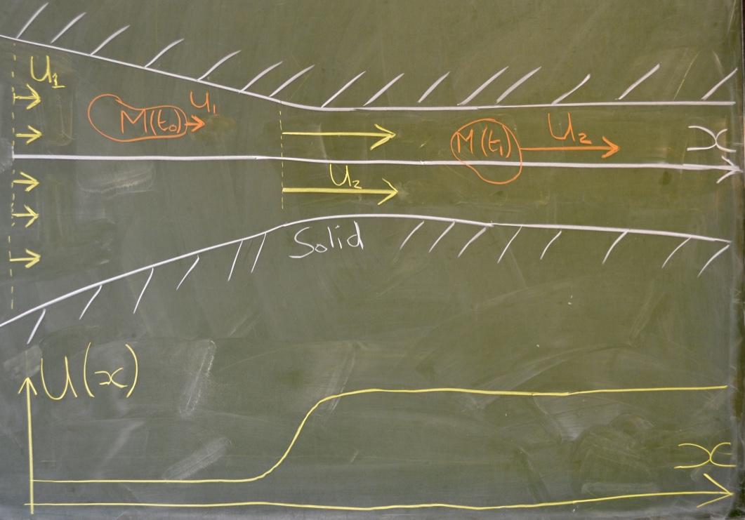
Example: If we take a one-dimensional steady flow (see Figure 2.5), then what is the acceleration of fluid particles?
| (2.6) |
so that where there is a spatial gradient in there is an acceleration.
2.4.5 Reynolds transport theorem
To describe laws of physics in terms of continuum quantities, we also need the time-rate-of-change of a total quantity enclosed within a finite Lagrangian volume . If the volumetric density of a property is , i.e., if the total amount of in any volume may written as
| (2.7) |
then
| (2.8) |
where is the bounding surface of and is the Eulerian velocity. The first term on the right hand side is simply the contribution that arises from the rate of change of within the volume, even when the Lagrangian volume stays fixed. The second term arises from the motion of the Lagrangian volume under the Eulerian velocity . Here is the rate at which volume of fluid enters the surface through an infinitesimal area (as shown in Figure 2.6), and its product with gives the amount of entering the volume per unit time.
2.5 Flow Visualisation
Watch the video on ‘Flow Visualisation’ narrated by Prof. Stephen J. Kline from Stanford University. YouTube link: www.youtube.com/watch?v=nuQyKGuXJOs, duration: 31 mins.
The most common way to visualise a flow, theoretically (once we have ) or experimentally, is by drawing a set of curves. Four types of curves are commonly used in fluid dynamics. Some are purely theoretical concepts, while others are used for experimental convenience.
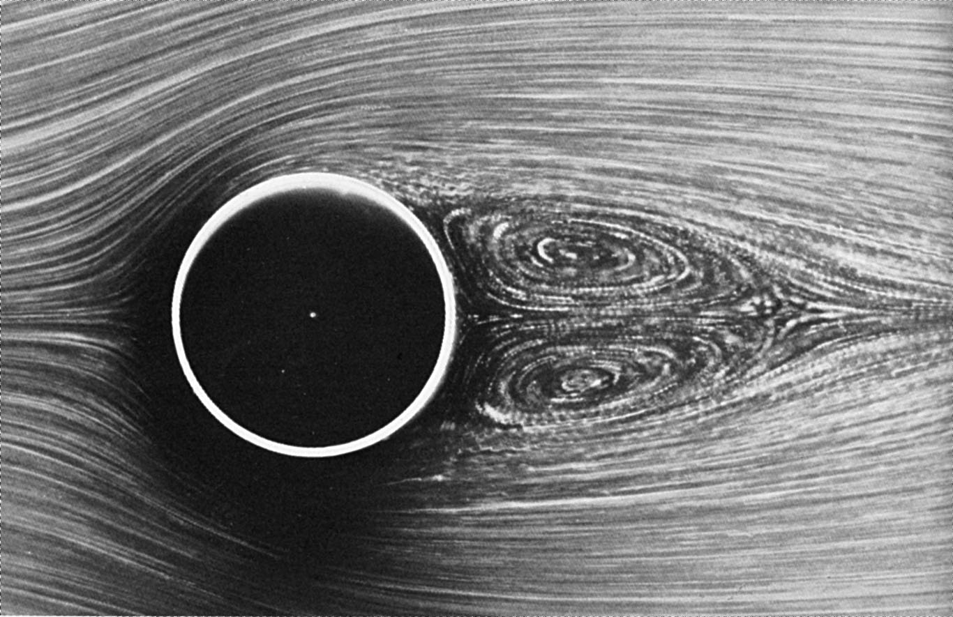
To visualise a flow field experimentally, one usually places illuminated passive tracers (e.g. dye, bubbles or beads that don’t alter the flow) into the flow (e.g. Figure 2.7). The various curves are then realized by the choice of the initial release of the tracer particles and the visualization technique.
-
1.
Particle paths or pathlines: The paths of fluid elements (‘particle paths’) , which are simply the locus of points traced by a Lagrangian fluid element. Equation (2.1) may be used to theoretically determine these from an Eulerian description of the velocity field. Typically a small amount of illuminated passive tracers are introduced in the flow, and the resulting images superimposed in post-processing to reveal the pathlines for a flow. Long exposures, if possible, also yield pathlines.
-
2.
Streaklines: The instantaneous locus of all the Lagrangian fluid elements that have passed through or will pass through a fixed point in space is a ‘streakline’. It is easier to visualize streaklines experimentally, which can be done by introducing a steady streak of a passive tracer in the fluid (hence the name). Theoretically, streakline at time passing through a point may be obtained by solving the equation
(2.9) for , where and are the initial and final times of interest, and then plotting for fixed while varying as a parameter.
-
3.
Timelines: A ‘time line’ is the subsequent shape of a curve made of Lagrangian fluid elements. It is more convenient to visualize a timeline experimentally than it is to calculate it theoretically. For the experimental visualization, a passive tracer is released at a time instance in the shape of a curve. The subsequent evolution of the curve naturally visualizes the timeline. To construct the timeline from an Eulerian velocity field, we start with a curve parameterized as by parameter . The subsequent shape of the curve at time is , which is the timeline at time .
-
4.
Streamlines: A ‘streamline’ is a curve which is everywhere tangent to the velocity vector of an Eulerian flow field. Streamlines are mathematical constructions, and, therefore, are easier to construct theoretically. Parameterized by an independent parameter , the streamlines at time are obtained by solving
(2.10) To visualize streamlines in an experiment, it is necessary to measure the Eulerian velocity field. This measurement can be accomplished using techniques such as particle image velocimetry (PIV).
Streamlines, although theoretical, have deep physical significance, especially for incompressible flows. Because the volume of a Lagrangian fluid element is conserved for an incompressible fluid, the only way a fluid element can move is by displacing the one ahead of it. At the same instance, the one ahead in turn displaces the one ahead of it, and so on. An incompressible fluid can flow only by forming such chains of instantaneous displacement of fluid elements. A streamline is nothing but one such chain.
Because of the aforementioned interpretation, streamlines cannot terminate in an incompressible fluid. They must extend all the way to infinity or form closed curves.
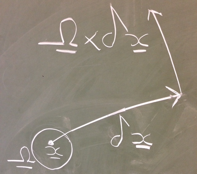
In general, the particle paths differ from the streamlines, which differ from streaklines. The following example illustrates that.
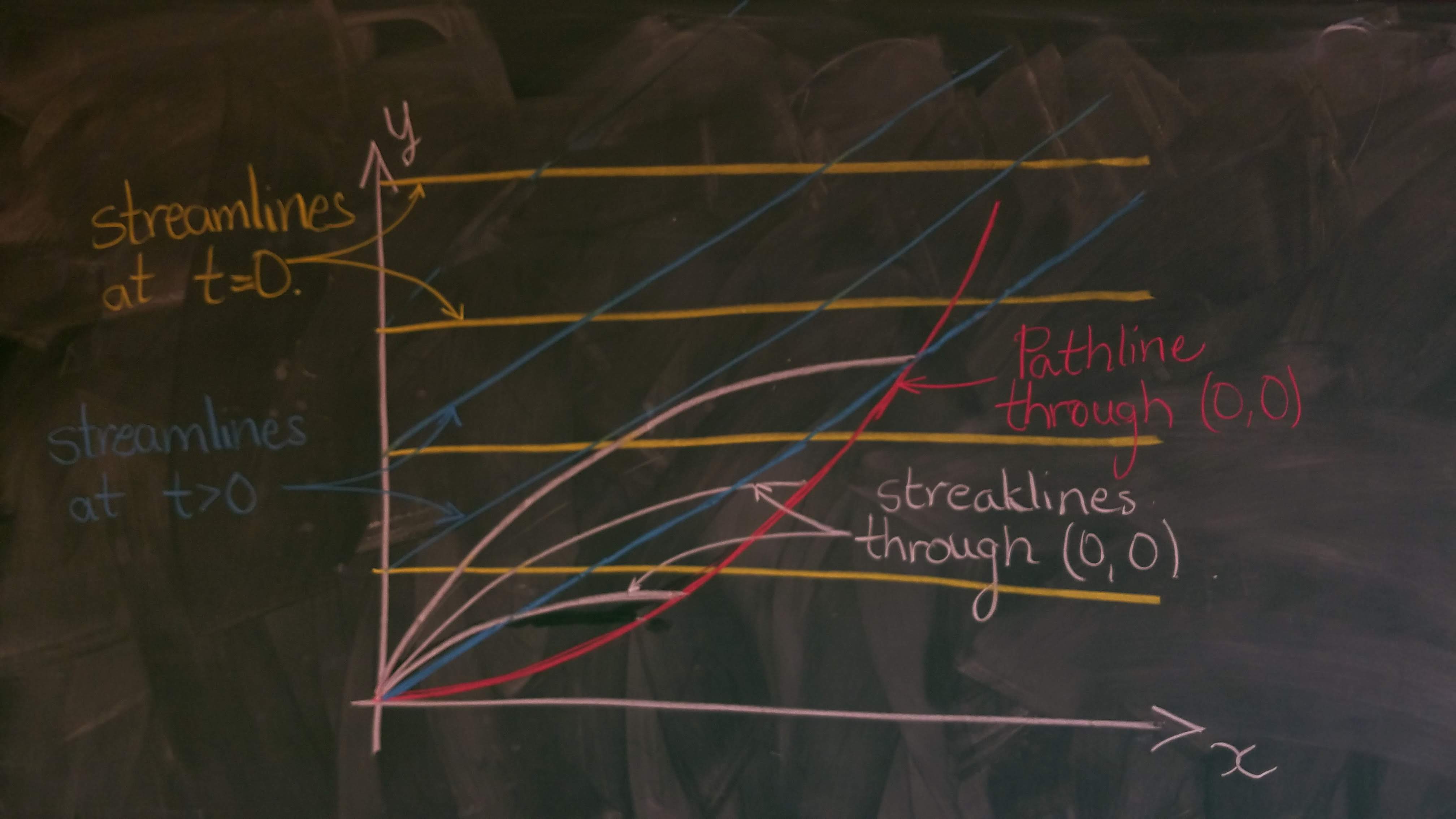
Example (from Acheson Ex 1.8): Consider the two-dimensional flow given by
What are the pathlines, streamlines and streaklines?
The pathlines are obtained from solving
for fixed initial position at . Therefore,
which, notably, could be used to transform from Eulerian to Lagrangian coordinates (by expressing in terms of . We can eliminate to find the particle paths
which are parabolas with their minimum at and as the coefficient of the quadratic term (see figure 2.8 for the pathline through the origin).
The streamlines come from
for a fixed . Therefore
for constant. Eliminating we find that
showing that the streamlines are straight lines whose slope will increase in time. The result is figure 2.8.
The streaklines are also easy to calculate. Upon solving equation (2.9), we get for
The equation for the curve for the streakline is , which is
These are to be plotted for fixed while varying as a parameter, which means that they are inverted parabolas through . The one through the origin is plotted in figure 2.8.
2.6 Deformation of infinitesimal fluid elements
The study of the deformation of continuous media (including solid and fluid dynamics) is a course in its own right, so we will only consider the concepts we will require to formulate the equations of fluid mechanics. In particular, we will attempt to understand how flow deforms fluid elements; as it is this (rate of) deformation that is related to the internal stress (and hence forces) required for formulating Newtons second law for the fluid.
The velocity can be decomposed into fundamental components which specify the kinematics of the flow (the geometry of the motion), i.e. how small fluid elements are deformed by the flow. To do so, consider the flow at an infinitesimal distance from a reference point , see figure 2.9.
The Taylor expansion of , keeping only the terms up to the first power in inclusive, gives
| (2.11) |
where we have decomposed into an anti-symmetric () rate of rotation tensor
and the symmetric () rate of strain tensor
Note that .
Each of the terms contributing to the velocity
| (2.12) |
can now be analysed. The first term in (2.11) is due to rigid body translation . If , then all fluid elements have the same velocity.
Rate of rotation OR Vorticity
Due to the antisymmetry of , there are only 3 independent components (all diagonal elements zero) and we can rewrite the term as a cross product or (see figure 2.11), where is the rate of rotation vector (you can check this). Thus we see that this term is associated with rigid body rotation about the reference point with rotational rate .
Notably, the rate of rotation vector is equal to half the vorticity vector
| (2.13) |
which is an important fluid mechanical quantity we will repeatedly encounter - now we can recognise it as a measure of the local rate of rotation in the fluid. In Cartesian coordinates it is given by
Example: How many components of vorticity does a 2D flow have?
For a two-dimensional flow , the vorticity has only one component where , with a rotation axis in the -direction.
Strain rate:
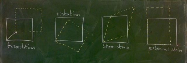
As the first two terms in (2.11) are associated with rigid body motion, it is the third term which represents the straining motions which distinguish the flow through the relative motion of adjacent fluid elements. The rate of strain tensor can be further decomposed into (a) diagonal elements which are associated with extensional motion and (b) off-diagonal elements give the shear rate of strain.
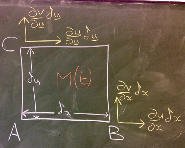
Consider how the components of deform an infinitesimal rectangular fluid element of size (figure 2.12) in a two-dimensional flow . For simplicity, we will remove translation of the fluid element by considering flow relative to the point , so that a Taylor expansion gives the flow components at adjacent points to shown in figure 2.12.
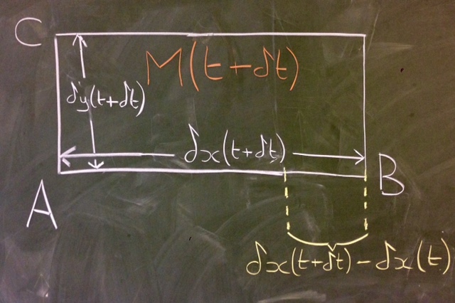
From figure (2.13) we can see that extensional rate of strain acts to increase the lengths of the sides. For example, taking the line , in a time the point B moves so that the new length of at time is
| (2.14) |
Therefore, the (infinitesimal) strain (extension/original length)
as expected.
It can be shown that the extensional components change the volume of the fluid element as
| (2.15) |
so that for an incompressible fluid, where the volume of the fluid element does not change in time (), we have . In other words, extension of a fluid element in one direction must lead to contraction in one of the other directions.
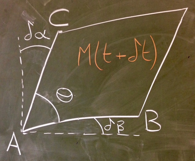
The shear rate of strain acts to drive the element from its rectangular shape. This can be quantified by measuring the angle between the sides. It can be shown that (see Examples Sheet 2) the angle at in figure 2.12 evolves according to
So we have seen that it is the vorticity and rate of strain that give us all of the information we require to understand how fluid elements are locally deformed, with the former telling us about the rotation of the flow and the latter about the relative motion of fluid elements (which is related to viscous stress).
Example (Adapted from Acheson §1.4): Consider the ‘shear flow’ . How does this simple flow deform fluid elements? E.g., what is the contribution from deformation to (2.12)?
Let’s consider all the different contributions to (2.12).
-
•
The translational term is just .
-
•
The vorticity will only have a component in the -direction which is
So there is rotation in the flow, despite the streamlines and particle paths being straight. This is because the velocity at the point is greater than that at so the line rotates clockwise (figure 2.14). The rate of rotation will be .
Therefore, the contribution to (2.12) is
-
•
The only non-zero entries in the rate of strain tensor will be due to . Therefore, extensional strains are all zero (ensuring incompressibility) and the only non-zero entries are . Consequently, the contribution to (2.12) is
-
•
Therefore, even in this simple flow there are rigid body motions of translation and rotation as well as deformation.
2.7 Conservation Laws in Continuum Mechanics
In continuum mechanics, it is customary to refer to laws of nature as conservation laws. An obvious example is the law of conservation of mass. As the fluid flows, mass can neither be created nor could it disappear. A less obvious one is Newton’s second law of motion. While momentum is not “conserved”, the law constrains the rate of change of momentum to be equal to force. Thus, by considering forces to be “sources” of momentum, one may still use the language of “conservation laws” to describe Newton’s second law. Examples of quantities to develop conservation laws for include mass, (linear) momentum, angular momentum (or moment of momentum), internal energy, total energy, and entropy. We will limit ourselves to mass, momentum and angular momentum.
Three main concepts need to be introduced to develop the conservation law for an abstract quantity, which we will call . These are the volumetric density of , the volumetric rate of generation (also known as the source) of , and the rate of exchange of between neighbouring fluid volumes.
1. Volumetric density of is the quantity such that the total amount of in any volume could be written as
Examples are presented in Table 2.1. The tensorial rank of and are identical. Furthermore, is an Eulerian field, i.e., .
| Notes | ||
|---|---|---|
| Mass | is the mass density | |
| Momentum | is the Eulerian fluid velocity | |
| Angular momentum | ||
| Internal energy | is the specific internal energy | |
| Entropy | is the specific entropy |
2. Volumetric source term also known as body source term, , is the volumetric density of the rate of generation of . The rate of increase of in any volume due to the volumetric source is
Examples include gravitational force as a source for momentum and ohmic generation of heat as an example for energy. The source is a field with its tensorial rank being equal to that of .
3. Surface source term, , originates from the fact that the volume may gain the quantity from the neighbouring fluid. For example, the force exerted on by the neighbouring fluid contributes to the rate of change of momentum in . By Newton’s third law, the volume exerts an equal and opposite force on the surrounding fluid. In this sense, the surface source may be interpreted as an exchange of between neighbouring fluid volumes.
A concrete example of such a term is the action of fluid pressure to generate force, or rate of change of momentum, on a volume . Due to the pressure, because the net force due to pressure is
Generally, the strength of such a surface source term is proportional to area of the bounding surface, rather than volume as for the volumetric source term. In general, the contribution to the rate of change of due to the surface source is written as
The tensorial rank of and of are equal. Clearly, must also be a field, i.e. . One important way differs from both and is that in addition to being a field, also has dependency on the orientation of the surface . In other words, if a point is on the boundary of two different volumes, can have different values depending on the unit outward normal to their bounding surfaces. This is represented through an explicit dependence on the unit normal as .
The conservation law for may now be written as
| (2.16) |
2.7.1 The dimensional inconsistency of the surface source term
Let us consider an arbitrary shape for . Now consider the limit of (2.16) as shrinks in size indefinitely, whilst retaining its shape. Let be a length characterizing . The volume of scales a and the area as . Thus, the first two terms of (2.16) scale as proportional to , while the surface source term scales proportional to , i.e.,
| (2.17) |
As the volume shrinks, becomes successively smaller, and relative to the surface source term, the first two terms become smaller. In the limit , the conservation law for (2.16) reduces to
| (2.18) |
In other words, for any infinitesimal volume, the contribution of the surface source term that is proportional to the area of the bounding surface must vanish. The consequence of this condition is the basis for all continuum mechanics.
2.7.2 Cauchy’s tetrahedron argument
Augustine-Louis Cauchy, a french mathematician, engineer and physicist, reasoned the compelling consequence of (2.18) by taking the shape of the volume to be a tetrahedron, as shown in Figure 2.15. The tetrahedron has four faces; the area of the inclined face is given by the (vector33 3 Reminder: the direction of a planar area is normal to its face.) , while the remaining three faces are , and , respectively, so that . We will now evaluate the terms of the integral in (2.18), but note because of the infinitesimal size of the tetrahedron, we will not need the distribution of over the areas. The value of may be considered a constant with , and we will drop the dependence on in the notation here. But because we could choose a tetrahedron of any proportions, the dependence on remains, which we will explicitly write.
The contribution to the integral in (2.18) from the four face may now be written as
| (2.19) |
By the principle of exchange of , , which arises from the fact that the amount of gained by the tetrahedron is lost by the neighbouring fluid. Let’s further define (in index notation) , where the on the indices of accounts for the free indices of , which may have a nonzero tensorial rank. In this way, has a tensorial rank one higher than . Furthermore, it follows from the geometry for tetrahedrons, . With this notation, (2.19) becomes
| (2.20) |
This dependence of the surface source term on the surface normal helps satisfies the condition (2.18) not only for a tetrahedron but also for any . This is so because
| (2.21) |
where the last step follows from the tensorial form of the divergence theorem. This step converts the surface integral to a volume integral, and in the limit of vanishing volume , this term scales as and not as .
The conservation law for now reads
| (2.22) |
Applying the Reynolds transport theorem and the divergence to the left hand side yields two additional forms of this equation.
| (2.23) | ||||
| (2.24) |
Equation (2.22-2.24) are integral representations of the law of conservation of . The term is the total flux of and is the convective flux. (In general, the flux of is the rate at which crosses a surface per unit area.) Conservation laws also have a differential form. To derive it, note that (2.24) holds irrespective of the volume . This is only possible if the integrand itself vanishes everywhere, i.e.,
| (2.25) |
We will see that in the differential representation of general conservation laws, the rate of change of the density is balanced by the divergence of the flux of and the volumetric generation of .
We now apply the result of this general analysis to specific quantities.
2.8 Conservation of Mass a.k.a. Mass Balance
Now we use the (classical) physical law that mass can neither be created or destroyed. This implies, when , then , and (2.22-2.24) becomes
| (2.26) | ||||
| (2.27) | ||||
| (2.28) |
Equations (2.26-2.28) are integral representations of the law of conservation of mass. The differential representation corresponding to (2.25)
| (2.29) |
We will now interpret the terms in some of representations of the law of conservation of mass, starting with (2.27). The first term in this equation is the rate of change of mass in a fixed (i.e. Eulerian) volume . The second term is the rate at which mass exits the volume due to the Eulerian velocity . Conservation of mass imples that the two rates must balance, which is the statement of (2.27).
Next we will discuss the terms in (2.29). The first term is the Eulerian rate-of-change of density the second is the divergence of the convective mass flux . Another form of (2.29), written using the expression
| (2.30) |
as
| (2.31) |
can be interpreted as the relative Lagrangian rate of change of density is balanced by the negative of the relative Lagrangian rate of change of volume. In other words, if volume of an infinitesimal Lagrangian element increases, its density must decrease.
If either the fluid or the flow is “incompressible”, that means that the density of infinitesimal Lagrangian fluid particles does not change with time, i.e., . This implies
| (2.32) |
2.9 Conservation of Momentum a.k.a. Momentum Balance
The density of momentum is , and its rate of change is a force as per Newton’s second law of motion. The volumetric source term is a force per unit volume that acts on the fluid and is termed a “body force”, e.g. the force of gravity. We will denote it by , where is acceleration due to the body force. Here the density and the volumetric source of momentum are vectors. The second rank tensor resulting from the surface force is the stress tensor, which when acting on an area element with normal exerts the force .
The three different integral forms representing conservation of momentum are
| (2.33) | ||||
| (2.34) | ||||
| (2.35) |
The differential form of momentum balance is
| (2.36) |
The left-hand side of (2.36) is can be simplified further by using the product rule and mass balance (2.29) as
| (2.37) |
This simplifies the differential form of momentum balance (2.36) to the Cauchy momentum balance equation as
| (2.38) |
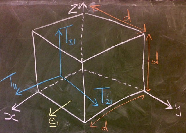
The left-hand side of this equation is mass times acceleration per unit volume of an infinitesimal Lagrangian element. The right-hand side contains the net forces on this volume per unit volume. It is obvious that is the body force per unit volume. To see that is the unbalanced surface force per unit volume, consider forces acting on a infinitesimal cubic fluid element with side and bottom corner at ; see figure 2.16. We will start with the -component of this force which will involve us calculating (with ) over all six sides of the cube.
| (2.39) | ||||
| (2.40) | ||||
| (2.41) |
Taylor expanding this expression in small and keeping the leading order only, we have:
where we have used the summation convention (with the repeated index).
Generalising to the other force components, we have:
symbolically this is the divergence of the stress tensor .
2.10 Conservation of Angular Momentum a.k.a. Torque Balance
The angular momentum changes at a rate equal to the net external torque applied on a body. For angular momentum, , , and . Note that the sources of angular momentum are related to the sources of linear momentum. We will go straight to the differential form of the angular momentum balance, which reads
| (2.42) |
Differentiating each term using the product rule yields
| (2.43) |
The first term is the cross product of with the linear momentum equation (2.36), and the second term is zero due to the anti-symmetry of in the indices and the symmetry of . Thus the only remaining term is . A direct consequence of this is that , or, in other words, is a symmetric second-rank tensor.
2.11 Constitutive laws
The differential equations governing a continuum material in an Eulerian description that we have derived so far are mass balance (2.29) and momentum balance (2.38). These equations are partial differential equations for determining the density and velocity by integrating in time, i.e., if suitable initial conditions are available for and , and the volumetric forces and stress were known, then one may use these equations to find the rate of change of and , which one then uses to determine the subsequent evolution of and . The situation is similar to the use of Newton’s second law of motion for describing the motion of rigid bodies; knowing the external forces one uses it to integrate for velocity and position. Here we think about integrating for and . Let’s examine quantities we do not know yet; viz. and .
The simplest one is : it must be prescribed as part of the problem.
The stress needs to determined based on the fluid and the flow, so that the system of equations (2.29) and (2.38) is closed. The closure of this system is made by the constitutive law for the continuum material. This constitutive law is what distinguishes between a solid and a fluid, and for that matter, between different kinds of “complex” fluids. Next we present some considerations for a constitutive law.
2.11.1 General considerations
An infinitesimal fluid element must continue to deform when a shear stress acts on it – this is the definition of a fluid. Therefore, we expect the components of the stress to be related to the components of the rate of shear tensor, i.e.,
| (2.44) |
We will start with some simple models.
2.11.2 An Ideal or Inviscid fluid
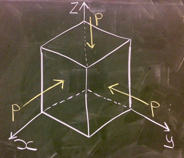
In an ideal or inviscid fluid there is no friction between fluid elements, so that the stress is given by an isotropic pressure that acts normal to the surface and inward. Therefore, our particular form of the stress tensor (known as a constitutive relation) is
| (2.45) |
Substituting into Cauchy’s equation (2.38), we arrive at the so-called Euler equation which describes inviscid fluid flow
| (2.46) |
This equation is named after Leonhard Euler, the celebrated Swiss mathematician.
Here the pressure is a thermodynamic quantity, so an equation of state that relates to other thermodynamic quantities would serve this purpose. The problem is that thermodynamic relations also introduce some other thermodynamic variable independent of density (say temperature) into consideration, which in itself could be non-uniformly distributed throughout the fluid. So an equation incorporating the law of conservation of thermal energy must be derived and treated for this new variable with mass and momentum balance. In some limited but practically useful circumstances, it is possible to eliminate the temperature and simply write . Examples include the propagation of sound waves. Under those circumstances, is well-defined. A very singular special case of this scenario is for an incompressible flow, for which is a constant, and, therefore, there is no explicit form for but must be deduced such that no changes in occur.
We will see later that an ideal fluid has a zero Newtonian viscosity.
In the absence of fluid motion we recover a hydrostatic balance .
2.11.3 A Newtonian Fluid
To describe a viscous fluid, we separate the pressure contribution to the stress tensor from the remaining terms — the latter will be associated with an internal friction or viscosity as
| (2.47) |
where is called the deviatoric stress tensor. For a Newtonian fluid, the deviatoric stress arises from viscosity, and therefore, is also called the viscous stress tensor. An ideal fluid is characterized by . For a general fluid the dependence on the rate-of-strain tensor in (2.44) is passed on to as for some tensorial function .
The Newtonian constitutive law corresponds to the relation where the relation between and is linear and isotropic. Linearity means that
| (2.48) |
where is a constant fourth rank tensor. For the relation to be isotropic, must be isotropic, i.e., it’s components may not depend of the coordinate system used to represent the tensor. We saw in (1.12c) that the most general fourth rank isotropic tensor has the form , where , and are scalar constants. Substituting in (2.48) yields . Here we learn that, in general, two constants are needed to specify the Newtonian constitutive law. However, for incompressible fluids (which Newton tacitly assumed), the term is identically zero, and setting to , where is the coefficient of Newtonian viscosity, yields the tensorial form of the Newtonian constitutive law for an incompressible fluid44 4 For a compressible flow, where can depend both on and the identity tensor, the most general form of such a tensor is (2.49) where is the viscosity (‘shear viscosity’ or ‘first viscosity coefficient’), is the “bulk viscosity” or the “second viscosity coefficient”.
| (2.50) |
Under a uniform shear flow, such as in Figure 2.1, the relation (2.50) reduces to the one-dimensional relation .
2.11.4 Navier-Stokes in cylindrical coordinates
The incompressible form of momentum conservation for the radial, azimuthal and axial components of velocity in a cylindrical polar coordinate system in differential form are:
| (2.52a) | ||||
| (2.52b) | ||||
| (2.52c) |
and the mass conservation equations is
| (2.53) |
Here , and are the , and components of gravitational acceleration.
2.12 Boundary and initial conditions
As usual for PDEs, in order to find a unique solution one has to specify appropriate boundary conditions and initial conditions.
2.12.1 Initial conditions
The set of relevant fields must be specified at at each point in the domain occupied by the fluid. For incompressible fluids, one only has to specify the initial velocity field
| (2.54) |
2.12.2 Boundary conditions
The number of boundary conditions required depends on the bulk equations (Euler or Navier Stokes in our case) and their form is determined by the properties of the boundaries (i.e. the physics at the boundary).
Viscous Fluids
At solid impenetrable boundaries, it has been found empirically that the fluid velocity at the boundary of the retaining volume adjusts itself to the boundary’s velocity : this is the famous no-slip boundary condition:
| (2.55) |
Inviscid Fluids
For inviscid fluids, where one only has first derivatives of fluid velocity (no term), one can only enforce inpenetrability of the boundary, i.e. that the normal to the boundary velocity component has to match to the one of the boundary, whereas the parallel velocity component remains arbitrary, since the fluid can slip freely along the boundary in the absence of internal friction. This is the so-called free-slip boundary conditions written as
| (2.56) |
In addition, at every point on the fluid where the fluid flows inward, the vorticity needs to be specified. This is an advanced condition, which we will not pursue in this course.
Kinematic boundary condition for moving material boundaries
For cases like the free surface, the motion of the boundary itself occurs under the influence of the fluid flow. In other words, the reason the free surface changes shape is because the fluid particles at the free surface flow. Mathematically, the free surface is a material boundary, i.e.,
| (2.57) |
Traction condition or the dynamic boundary condition
In lieu of specifying velocity, one may also specify the traction , i.e. the force per unit area on the boundary. In general, the traction condition is written as
| (2.58) |
This condition is especially useful for moving free surfaces, where two conditions are needed, viz., one for specifying the rate of motion of the interface and another as a boundary condition for the fluid partial differential equations. In that case, along with the kinematic boundary condition, the traction information furnishes the second condition.