Chapter 6 Potential flow
The case where the fluid velocity in given by
| (6.1) |
is called potential flow. Velocity profiles of this type arise in a number of situations in practice, but most importantly this theory allows fluid dynamicists to construct flow profiles that automatically satisfy conservation of mass and momentum. Here we treat this subject.
6.1 Conditions for and implications of potential flow
The conditions under which potential flow is realized are those of incompressibility and irrotationality, i.e.,
| (6.2) |
A necessary and sufficient condition for irrotationality is
| (6.3) |
where is a scalar field known as the velocity potential. Substituting this form of into the incompressibility conditions yields Laplace equation for . In this way, mass is conserved.
We have seen in (5.11), that momentum is conserved if the pressure satisfies the Bernoulli equation, i.e.,
| (6.4) |
In this manner, potential flow satisfies mass and momentum conservation for a viscous fluid.
To construct a potential flow, one solves the Laplace equation (6.1) for subject to appropriate boundary conditions. Given the nature of Laplace equation, on the boundaries only one of the two components of velocity may be imposed, but not both. On the boundary between the fluid and a solid object, a condition of no-normal flow is imposed, i.e.,
| (6.5) |
Therefore, in general, the no-slip condition cannot be satisfied by potential flow past solid objects and potential flow generally slips past the walls. Regardless, potential flow is incredibly succcessful in providing insight into situations where solid bodies are either not present or could be abstracted away.
6.2 Incompressible and irrotational flow in two-dimensions
While the general concept of potential flow applies in three dimensions, the application of complex variables makes potential flow much more powerful in two dimensions. Essentially, the use of complex variables trivializes the solution of Laplace equation. The only remaining complexity that remains is the satisfaction of the boundary conditions. In the rest of this chapter, we will focus on two-dimensional incompressible irrotational flow.
Irrotationality in two dimension implies for the components of velocity
| (6.6) |
Similarly, incompressibility implies
| (6.7) |
where is a field called stream function.
This type of reciprocal relation between the deriviatives of two scalar functions, in our case and , are called the Cauchy-Reimann conditions:
| (6.8) |
Owing to this relation, both and satisfy Laplace equation, i.e., . Furthermore, and are the real and imaginary part of a holomorphic function of the complex variable , i.e.
| (6.9) |
Thus, the strategy for generating potential flows is to construct holomorphic functions called complex potentials that satisfy the necessary boundary condition. The fluid velocity is given by the relation
| (6.10) |
Here are some geometric relations between , and streamlines.
6.2.1 Stream function and streamlines
Contours of constant stream function are streamlines of the flow. To see this, consider the directional derivative of the stream function in the direction of the streamline, i.e. in the direction of velocity
| (6.11) |
Thus, irrespective of location in the flow, does not vary in the direction of streamlines. Therefore, is a constant along a streamline. In other words, streamlines are contours of constant stream function.
6.2.2 Stream function and velocity potential
Contours of constant stream function and those of constant velocity potential meet orthogonally. To see this, consider the dot product of and , the normals of the contours at a given point:
| (6.12) |
Since the normals are orthogonal, the tangents must be too, and therefore the curves must be too.
6.3 Elementary complex potentials
Some basic elements that are used to construct the complex potentials.
6.3.1 Uniform flow
Consider the complex potential
| (6.13) |
The flow velocity corresponding to this potential is
| (6.14) |
i.e., a uniform flow at an angle to the -axis. An example of this flow is shown in Figure 6.1(a).
6.3.2 Point source
Consider the complex potential
| (6.15) |
where is the polar representation of the complex variable . The flow velocity corresponding to this potential is
| (6.16) |
i.e., a radially outward flow decaying inversely proportional with distance. An example of this flow is shown in Figure 6.1(b). For what follows, let and .
To understand why the flow corresponding to this potential is termed as the point source, consider the divergence and curl of the velocity field:
| (6.17) | |||
| (6.18) |
for , but this calculation says nothing about . To deduce that, consider the line integrals along the circle of radius
| (6.19) | |||
| (6.20) |
where and are the unit normal and tangential vectors to the curve . Given that, due to the divergence and Stokes theorems, respectively,
| (6.21) | |||
| (6.22) |
the inesacapable conclusion is that for this flow , where is the Dirac-delta function and . Thus, this flow is irrotational everywhere, but incompressible only for . Volume is not conserved at , but instead is generated there. Hence the terminology to describe this flow as a “point source”.
6.3.3 Point vortex
Consider the complex potential
| (6.23) |
The flow velocity corresponding to this potential is
| (6.24) |
i.e., an azimuthal flow decaying inversely proportional with distance. An example of this flow is shown in Figure 6.1(c).
We again examine and to understand the terminology associated with this flow. Just as for the point source,
| (6.25) | |||
| (6.26) |
for , but which says nothing about . The line integrals along the circle of radius
| (6.27) | |||
| (6.28) |
which, in view of (6.21-6.22) lead to the inescable conclusion that the flow is incompressible everywhere but irrotational only for . The vorticity is, in fact, . Hence the flow due to this potential is termed as the “point vortex”.
6.3.4 Point dipole
The flow constructed by the linear superposition of a point source and an equal point sink (i.e., a source with negative strength) located vanishingly small distances apart constitutes a point dipole. The complex potential is constructed as
| (6.29) |
Of course, in the limit , the potential would vanish, unless the source-sink pair also strengthened in the process. In particular, let , so that the source-sink pair strength is inversely proportional to the distance between them. Here is the strength of the point dipole. With this assumption,
| (6.30) |
The flow due to the point dipole is depicted in Figure 6.1(d). The streamlines and equipotential lines are both sets of circles that are tangential to the and axes, respectively, at the origin.
6.3.5 Higher multipoles
Note that, due to its construction, the potential due to a point dipole is the derivative of the potential due to a point source. This can be extended to higher orders called “multipoles”. For example, a point quadrupole is a point dipole of point dipoles with a complex potential proportional to . And octupole is a point dipole of quadrupoles with potential . And so on.
In this manner, the general complex potential with the farfield approaching uniform flow may be written as
| (6.31) |
Here, the coefficients , , , , , etc, may be functions of time.
6.4 Potential flow past immersed bodies
The coefficients , , , , …, may be chosen to construct the complex potential for flow past bodies. Here are some examples.
6.4.1 Rankine half-body
The linear superposition of a uniform flow and a point source may be used to represent flow past a semi-infinite body, called the Rankine half-body. The complex potential is
| (6.32) |
The flow streamlines and equipotential lines are shown in Figure 6.2(a).
Any region of the plane on one side of a streamline may be replaced by a solid body and the complex potential in the remaining region describs potential flow past this solid body. For example, consider the streamline given by , where
| (6.33) |
The streamline is shown in Figure 6.2(b) and the area inside the streamline, shaded blue in the figure, is the Rankine half-body. The complex potential in (6.32) describes the flow past this Rankine half-body.
6.4.2 Rankine oval
The linear superposition of a uniform flow, a point source and a point sink may be used to represent flow past a finite body, called the Rankine oval. The complex potential is
| (6.34) |
The flow streamlines and equipotential lines are shown in Figure 6.3(a).
6.4.3 Circle
The Rankine oval approaches a circle as the source and the sink approach each other to form a dipole. The complex potential in this case is
| (6.36) |
The flow streamlines and equipotential lines are shown in Figure 6.4(a).
Consider the streamline given by , where
| (6.37) |
The streamline is shown in Figure 6.4(b) and the area inside the streamline, shaded blue in the figure, is a circle of radius . The complex potential in (6.36) describes the flow past this circle.
An arbitrary point vortex centered at the center of the circle may be added to the mix without violating the boundary condition on the circle. The most general potential flow around a circle is given by
| (6.38) |
Here is the circulation around the circle, perhaps due to the spinning of the circle. The flow due to this potential is shown in Figure 6.4(c).
6.5 Force on a immersed body
The force on the body due to the potential flow (6.31) may be calculated by integrating the force due to the fluid pressure. The force on the body per unit length out of the plane of the paper is
| (6.39) |
where is the bounding closed streamline defining the body. The fluid pressure is determined by Bernoulli equations as
| (6.40) |
The contribution to the force due to gravity is the force of buoyancy from Archimedes principle. Here we calculate the contribution from the remaining two terms.
6.5.1 Force in a steady potential flow
In steady potential flow, only the term contributes to the net unbalanced force beyond buoyancy. In complex variables, let the components of the force be written as . If the tangent to makes an angle to the -axis, then because the flow is tangential to the streamline. Also, because the components of velocity are , . The product of the unit normal and the infinitesimal line element is . The complex conjugate of the force is
| (6.41) |
where the complex integration infinitesimal .
Using this expression for force, and substituting (6.31) in (6.41) yields
| (6.42) |
where Cauchy’s residue theorem is employed for calculating the contour integral. Law of conservation of mass demands that for a body immersed in the flow , and therefore,
| (6.43) |
The drag on an object is the force it experiences in the direction of the flow, while the lift is the force perpendicular to the flow. According to (6.43), the lift on an immersed body due to the potential flow is , which is the statement of the Kutta-Joukowsky (also spelled Joukowski, Zhukowski or Zhukovsky) theorem in aerodynamics. The lift on the spinning circle, due to this theorem, is .
The fact that a body immersed in a potential flow does not experience any drag is the subject of the D’Alembert paradox. Neither the Rankine oval, nor the circle, nor body of any other shape experiences any drag in potential flow. D’Alembert paradox exist because potential flow does not satisfy the no-slip condition. The friction of a viscous fluid with the solid boundary generates vorticity, which is transported by the fluid to regions away from the immersed body. In this manner, application of the no-slip boundary condition on viscous fluids invalidates the assumptions underlying potential flow, especially that the flow be irrotational. In fact, the shedding of vorticity into the flow is the origin of fluid dynamical drag (this we state without proof at this point).
6.5.2 Added mass from the unsteady term
Consider the contribution of the term . The resulting force is
| (6.44) |
Let us examine this expression for the case of flow around a circle, so that is given by (6.36). This corresponds to
| (6.45) |
The integral for force yields
| (6.46) |
This result may be interpreted in the following way. Any acceleration of the circle implies an acceleration of the fluid around it. This acceleration needs an additional force proportional to the acceleration. The coeffient of proportionality between this additional force and the acceleration is the “added mass” the fluid presents to the motion of the circle. In this case, the added mass in .
6.6 Flow around an airfoil
The lift generated by an airfoil is a central result in aerodynamics, which makes use of potential flow.
Some salient features of this flow are visualized in Figure 6.5. The stagnation streamline is incident on the lower surface of the airfoil, which develops the stagnation pressure under the airfoil. The streamlines curve around the leading edge of the airfoil, generating a low-pressure area above the airfoil. Finally and crucially, note that the stagnation streamline separates from the plate at the trailing edge. These are the features that will guide us in constructing the appropriate potential flow.
Here we will present one calculation, that of the lift on the prototypical airfoil – a flat plate, which hightlights this central result. The underlying potential flow is constructed in this case using a technique known as conformal mapping (the same technique can be used to construct flow around airfoils of other shapes).
A conformal map is a map between two complex variables, which we take to be and . Here corresponds to the physical spatial variable, in which the flat plate exists, and is the mapped variable, in which the flat plate is mapped to a circle. The particular map we use is called the Joukowsky map:
| (6.47) |
A circle in -plane, is mapped to
| (6.48) |
which is an ellipse of major axis along the -axis and minor axis along the -axis. In the limit , the ellipse approaches a flat plate . The point is mapped to the trailing edge of the plate . The chord of the flat plate is .
While it is possible to solve for the inverse map in closed form, the idea is to not need the explicit expression for the inverse. However, we do need the inverse map to be analytic so that the complex potential
| (6.49) |
automatically deforms the streamlines and converts the circular streamine in the coordinates to be a flat plate in the coordinates, whilst preserving the analyticity of the complex potential.
We start with the complex potential (6.38) for flow around a circle, but now expressed in and with an angle of attack , i.e.,
| (6.50) |
As , the largest term in is , corresponding with uniform flow at an angle to the flat plate. The complex velocity in the plane is
| (6.51) |
The velocity in the -coordinates is
| (6.52) |
As , approaches .
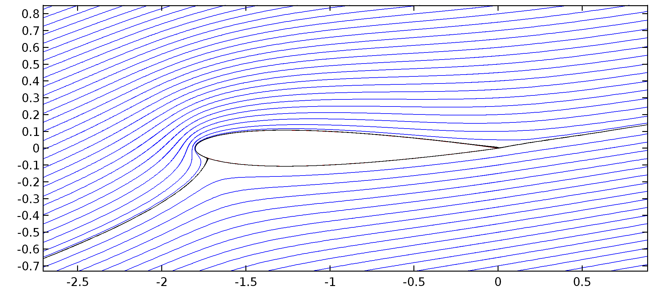
Consider the case . An example of the flow corresponding to this case is shown in Figure 6.6. Note that the stagnation point in the -plane is at . This point maps in the -plane to below the flat plate, and above it. Note that in this flow, the stagnation streamline does not separate from the trailing edge .
The stagnation point may be moved by judiciously choosing the value of . The condition that the trailing edge be the rear stagnation point is called the Kutta condition. We impose the Kutta condition by ensuring that the stagnation point in the -coordinates is at . Substituting the velocity at yields
| (6.53) |
The streamlines and equipotential lines corresponding to the value of that enforces the Kutta condition, shown in Figure 6.7, illustrate this condition.
The lift on the falt-plate is given by
| (6.54) |
This result can be converted to a dimensionless form in terms of the coefficient of lift, , defined as
| (6.55) |
Using the result (6.54), the lift coefficient depends on the angle of attack as
| (6.56) |
Figure 6.8 shows that the results of (6.56) compare well with the lift coefficient computed using the commercial software COMSOL for small . The agreement worsens around due to a phenomenon called stall, in which the stagnation streamline also separates from the leading edge. A careful treatment of the influence of viscosity is needed to gain a deeper understanding of stall.