Chapter 13 Linear waves and instabilities

The equations governing the flow and interface shape are as follows. Because both the static water and uniformly flowing air initially lack vorticity, and viscosity and non-conservative forces needed for generating vorticity in the flow are absent, the flow remains irrotational in both fluids.

1. 1.

   Air: The fluid velocity ${𝒖}_a$, the velocity potential ${\varphi }_a$ and the fluid pressure $p_a$ satisfy

   	${𝒖}_a=\mathbf{\nabla }{\varphi }_a,\text{and}\mathbf{\nabla }\cdot {𝒖}_a=0\to {\nabla }^2{\varphi }_a=0,$		(13.1a)
   	${\rho }_a\left({\displaystyle \frac{\partial {\varphi }_a}{\partial t}}+{\displaystyle \frac{1}{2}}{|\mathbf{\nabla }{\varphi }_a|}^2\right)+p_a+{\rho }_{a}gy=c=\text{a constant},$		(13.1b)

   where (13.1a) represents conservation of mass and (13.1b) conservation of meomentum in the form of Bernoulli equation for unsteady potential flow, as described in (5.11) from §5.2.2.

2. 2.

   Water: Denoting the water velocity, velocity potential and pressure by ${𝒖}_w$, ${\varphi }_w$ and $p_w$, the equations governing its flow analogous to the ones in the air are

   	${𝒖}_w=\mathbf{\nabla }{\varphi }_w,\text{and}\mathbf{\nabla }\cdot {𝒖}_w=0\to {\nabla }^2{\varphi }_w=0,$		(13.2a)
   	${\rho }_w\left({\displaystyle \frac{\partial {\varphi }_w}{\partial t}}+{\displaystyle \frac{1}{2}}{|\mathbf{\nabla }{\varphi }_w|}^2\right)+p_w+{\rho }_{w}gy=d=\text{another constant}.$		(13.2b)

3. 3.

   Dynamic boundary condition: At the interface, the force per unit area exerted from the two fluids must add up to the unbalanced force due to Laplace pressure (Refer to: Chapter on surface tension) on the interface. Mathematically, this amounts to the boundary condition at $y=h$ as

   $p_a=p_w+\sigma \kappa ,\text{where}\kappa =\left({\displaystyle \frac{{\partial }^{2}h/\partial x^2}{1+{\left(\partial h/\partial x\right)}^{3/2}}}\right)=\text{interface mean curvature}.$

   (13.3)

   This condition imposes momentum balance over the interface and ensures that forces are transmitted appropriately across it.

4. 4.

   Kinematic boundary condition: The interface moves with the fluid(s) or, in other words, the interface is a “material property”. The corresponding mathematical statement is

   ${\displaystyle \frac{D}{Dt}}\left(h(x,t)-y\right)=0.$

   When the material derivative is expanded and the velocity of the two fluids is substituted, the kinematic boundary condition becomes

   	${\displaystyle \frac{\partial h}{\partial t}}+{\displaystyle \frac{\partial {\varphi }_a}{\partial x}}{\displaystyle \frac{\partial h}{\partial x}}={\displaystyle \frac{\partial {\varphi }_a}{\partial y}}\text{at}y=h,\text{and}$		(13.4a)
   	${\displaystyle \frac{\partial h}{\partial t}}+{\displaystyle \frac{\partial {\varphi }_w}{\partial x}}{\displaystyle \frac{\partial h}{\partial x}}={\displaystyle \frac{\partial {\varphi }_w}{\partial y}}\text{at}y=h,$		(13.4b)

   where (13.4a) uses the air velocity and (13.4b) uses the water velocity.

Equations (1-4) constitute the governing equations for the air-water-interface dynamics.

A trivial steady state satisfies of the governing equations:

	${𝒖}_a=U{𝒆}_x,$	${\varphi }_a=Ux,$	$p_a=c-{\rho }_{a}gy-{\displaystyle \frac{1}{2}}{\rho }_a{U}^2$	,		(13.5a)
	${𝒖}_w=\mathrm{𝟎},$	${\varphi }_w=0,$	$p_w=d-{\rho }_{w}gy,$			(13.5b)
	$h(x,t)=0.$					(13.5c)

This flow corresponds to a uniform flow in the air, no flow in the water and a flat interface. The configuration is perturbed slightly as

	${𝒖}_a=U{𝒆}_x+ϵ{𝒖}_a^{\prime },$	${\varphi }_a=Ux+ϵ{\varphi }_a^{\prime },$	$p_a=ϵp_a^{\prime }+c-{\rho }_{a}gy-{\displaystyle \frac{1}{2}}{\rho }_a{U}^2$	,		(13.6a)
	${𝒖}_w=\mathrm{𝟎}+ϵ{𝒖}_w^{\prime },$	${\varphi }_w=0+{\varphi }_w^{\prime },$	$p_w=ϵp_w^{\prime }+d-{\rho }_{w}gy,$			(13.6b)
	$h(x,t)=0+ϵh^{\prime }(x,t).$					(13.6c)

Here $ϵ$ parameterizes the size of the perturbation, and the functions decorated with a prime denote a perturbation to the unprimed version of the function. This transformation of the dependent variables adds little to the analysis by itself, except when the size of the perturbation is assumed to be small. Mathematically, this assumption implies a vanishingly small $ϵ$ and leads to the process of linearization as follows.

Substituting (13.1.2) in the governing equations (1-4) and canceling a factor of $ϵ$, and dropping the prime decoration leads to

	${𝒖}_a=\mathbf{\nabla }{\varphi }_a,\text{and}\mathbf{\nabla }\cdot {𝒖}_a=0\to {\nabla }^2{\varphi }_a=0,$		(13.7a)
	${\rho }_a\left({\displaystyle \frac{\partial {\varphi }_a}{\partial t}}+U{\displaystyle \frac{\partial {\varphi }_a}{\partial x}}+{\displaystyle \frac{ϵ}{2}}{|\mathbf{\nabla }{\varphi }_a|}^2\right)+p_a=0\text{at}y=ϵh,$		(13.7b)

from (1),

	${𝒖}_w=\mathbf{\nabla }{\varphi }_w,\text{and}\mathbf{\nabla }\cdot {𝒖}_w=0\to {\nabla }^2{\varphi }_w=0,$		(13.8a)
	${\rho }_w\left({\displaystyle \frac{\partial {\varphi }_w}{\partial t}}+{\displaystyle \frac{ϵ}{2}}{|\mathbf{\nabla }{\varphi }_w|}^2\right)+p_w+{\rho }_{w}gh=0\text{at}y=ϵh,$		(13.8b)

from (2),

$p_a-{\rho }_{a}gh=p_w-{\rho }_{w}gh+\sigma {\displaystyle \frac{{\partial }^{2}h/\partial x^2}{{\left(1+{ϵ}^2{(\partial h/\partial x)}^2\right)}^{3/2}}}\text{at}y=ϵh,$

(13.9)

from (13.3), and

	${\displaystyle \frac{\partial h}{\partial t}}+U{\displaystyle \frac{\partial h}{\partial x}}+ϵ{\displaystyle \frac{\partial {\varphi }_a}{\partial x}}{\displaystyle \frac{\partial h}{\partial x}}$	$={\displaystyle \frac{\partial {\varphi }_a}{\partial y}}\text{at}y=ϵh,\text{and}$		(13.10a)
	${\displaystyle \frac{\partial h}{\partial t}}+ϵ{\displaystyle \frac{\partial {\varphi }_w}{\partial x}}{\displaystyle \frac{\partial h}{\partial x}}$	$={\displaystyle \frac{\partial {\varphi }_w}{\partial y}}\text{at}y=ϵh,$		(13.10b)

from (4). Equations (13.1.2-13.1.2) are in every way equivalent to (1-4) so far. Now we apply the defining step of linearization, the limit os vanishingly small $ϵ$. Substituting this limit into (13.1.2-13.1.2) yields

	${𝒖}_a=\mathbf{\nabla }{\varphi }_a,\text{and}\mathbf{\nabla }\cdot {𝒖}_a=0\to {\nabla }^2{\varphi }_a=0,$		(13.11a)
	${\rho }_a\left({\displaystyle \frac{\partial {\varphi }_a}{\partial t}}+U{\displaystyle \frac{\partial {\varphi }_a}{\partial x}}\right)+p_a=0\text{at}y=0,$		(13.11b)

from (13.1.2),

	${𝒖}_w=\mathbf{\nabla }{\varphi }_w,\text{and}\mathbf{\nabla }\cdot {𝒖}_w=0\to {\nabla }^2{\varphi }_w=0,$		(13.12a)
	${\rho }_w\left({\displaystyle \frac{\partial {\varphi }_w}{\partial t}}\right)+p_w=0\text{at}y=0,$		(13.12b)

from (13.1.2),

$p_a-{\rho }_{a}gh=p_w-{\rho }_{w}gh+\sigma {\displaystyle \frac{{\partial }^{2}h}{\partial x^2}}\text{at}y=0,$

(13.13)

from (13.9), and

	${\displaystyle \frac{\partial h}{\partial t}}+U{\displaystyle \frac{\partial h}{\partial x}}$	$={\displaystyle \frac{\partial {\varphi }_a}{\partial y}}\text{at}y=0\text{and}$		(13.14a)
	${\displaystyle \frac{\partial h}{\partial t}}$	$={\displaystyle \frac{\partial {\varphi }_w}{\partial y}}\text{at}y=0,$		(13.14b)

from (13.1.2). A defining feature of the resulting (13.1.2-13.1.2) is that they are linear in the dependent variables. Hence this process of making infinitesimally small amplitude perturbations is called linearization. Also note, how the boundary conditions are now imposed at $y=0$ instead of the exact interface location $y=ϵh$.

The most convenient way to interpret the linear equations (13.1.2-13.1.2) is to identify the directions along which translational invariance applies and perform a Fourier transform along them. In this case, the physical system and the corresponding mathematical model given by (13.1.2-13.1.2) is translationally invariant along $x$ (but not $y$ because of the presence of the interface). A shift of the origin along $x$ does not change the equations, but a shift along $y$ does through a change in the nominal position of the interface. Thus, we will perform a Fourier transform of (13.1.2-13.1.2) along the $x$ axis.

For this purpose, let us define the transformed variable $\widehat{\varphi }$ decorated by a caret for the untransformed undecorated variable $\varphi$

	$\widehat{\varphi }(k,y,t)$	$={\displaystyle \frac{1}{2\pi }}{\displaystyle {\int }_{-\mathrm{\infty }}^{\mathrm{\infty }}}\varphi (x,y,t)e^{-ikx}\text{d}x,\text{and}$		(13.15a)
	$\varphi (x,y,t)$	$={\displaystyle {\int }_{-\mathrm{\infty }}^{\mathrm{\infty }}}\widehat{\varphi }(k,y,t)e^{ikx}\text{d}k.$		(13.15b)

Here (13.15a) is the forward Fourier transform and (13.15b) is the inverse transform. The transform is a function of the variable $k$, which is called the wave number. And interpretation of (13.15b) is that the function in the physical space $\varphi (x,y,t)$ is being written as a linear combination of the sinusoids, i.e. $e^{ikx}$, of wavenumber $k$ (equivalently wavelength $2\pi /k$) with amplitude $\widehat{\varphi }(k,y,t)$. Thus the forward transform (13.15a) decomposes a given function into its components and deduces the amplitude of the sinusoid with wavelength $2\pi /k$. The amplitudes are in general complex, which accounts for the sine and the cosine part of the sinusoid. However, because the variable $\varphi (x,y,t)$ in the physical space is real, the Fourier transformed amplitude $\widehat{\varphi }(k,y,t)$ satisfies $\widehat{\varphi }(-k,y,t)={\widehat{\varphi }}^{*}(k,y,t)$, where the asterisk denotes complex conjugation.

A property of the Fourier transform used in this analysis is the relation between the Fourier transform of functions and its derivatives. It may be readily verified using integration by parts that

$ik\widehat{\varphi }(k,y,t)$

$={\displaystyle \frac{1}{2\pi }}{\displaystyle {\int }_{-\mathrm{\infty }}^{\mathrm{\infty }}}{\displaystyle \frac{\partial \varphi (x,y,t)}{\partial x}}{e}^{-ikx}\text{d}x.$

(13.16)

Loosely speaking, differentiation with respect to $x$ in the real space is converted to a factor of $ik$ is Fourier transformed space.

Fourier transform of (13.1.2-13.1.2) and dropping the caret decoration yields

	$u_a=ik{\varphi }_a,v_a={\displaystyle \frac{\partial {\varphi }_a}{\partial y}},\text{and}ik{u}_a+{\displaystyle \frac{\partial v_a}{\partial y}}=0\to \left({\displaystyle \frac{{\partial }^2}{\partial y^2}}-k^2\right){\varphi }_a=0,$		(13.17a)
	${\rho }_a\left({\displaystyle \frac{\partial {\varphi }_a}{\partial t}}+ikU{\varphi }_a\right)+p_a=0\text{at}y=0,$		(13.17b)

from (13.1.2),

	$u_w=ik{\varphi }_w,v_w={\displaystyle \frac{\partial {\varphi }_w}{\partial y}},\text{and}ik{u}_w+{\displaystyle \frac{\partial v_w}{\partial y}}=0\to \left({\displaystyle \frac{{\partial }^2}{\partial y^2}}-k^2\right){\varphi }_w=0,$		(13.18a)
	${\rho }_w{\displaystyle \frac{\partial {\varphi }_w}{\partial t}}+p_w=0\text{at}y=0,$		(13.18b)

from (13.1.2),

$p_a-{\rho }_{a}gh=p_w-{\rho }_{w}hg-\sigma k^{2}h\text{at}y=0,$

(13.19)

from (13.13), and

	${\displaystyle \frac{\partial h}{\partial t}}+ikUh$	$={\displaystyle \frac{\partial {\varphi }_a}{\partial y}}\text{at}y=0\text{and}$		(13.20a)
	${\displaystyle \frac{\partial h}{\partial t}}$	$={\displaystyle \frac{\partial {\varphi }_w}{\partial y}}\text{at}y=0,$		(13.20b)

from (13.1.2). Equations (13.1.3-13.1.3) are the Fourier transformed versions governing the evolution of the perturbation. Notably, the amplitudes ${\varphi }_a$, ${\varphi }_w$, $p_a$, $p_w$ and $h$ with wavenumber $k$ evolve independently of other wavenumbers, as inferred from the fact that (13.1.3-13.1.3) do not couple the wavenumber $k$ to any other wavenumber. This demonstrates that a sinusoidal perturbation with wavenumber $k$ evolves in time independently of ever other wavenumber that may comprise the general perturbation. Because the most general perturbation can always be decomposed into its constituent sinusoids using the Fourier transform, each wavenumber then evolved in time independently, and later recomposed using the inverse Fourier transform. Thus, it suffices to study the evolution of each wavenumber separately.

(Sinusoids are normal modes – i.e. shape functions which decouple a linear operator – for translationally invariant systems. If the system of interest is not translationally invariant, the normal modes for that system may be deduced by solving for the eigenfunctions of the underlying linear operator. Because the process of investigating the evolution of small perturbation leads to linear equations, determining normal modes of the underlying linear operators are a common operation in the analysis of waves and instabilities.)

The solution to (13.17a) for ${\varphi }_a$ and (13.18a) for ${\varphi }_w$ is

	${\varphi }_a$	$=A{e}^{-|k|y}+B{e}^{|k|y}\text{for }y>0\text{ and}$		(13.21a)
	${\varphi }_w$			(13.21b)

where $A$, $B$, $C$ and $D$ are constants of integration, themselves functions of $k$ and $t$. Now we apply the conditions of stagnancy deep into the water layer, and uniform flow high up into the air layer. This implies that the perturbation to velocity perturbations decay as $|y|\to \mathrm{\infty }$. This is achieved by setting the constants $B=D=0$. The remaining constants $A$ and $C$ are determined by the boundary conditions on the interface $y=0$. Substituting in (13.1.3-13.1.3) then yields a set of five coupled equations for $A$, $C$, $p_a$, $p_w$ and $h$ as

	$p_a$	$=-{\rho }_a\left({\displaystyle \frac{\partial }{\partial t}}+ikU\right)A,$		(13.22a)
	$p_w$	$=-{\rho }_w{\displaystyle \frac{\partial C}{\partial t}},$		(13.22b)
	$p_a-p_w$	$=-({\rho }_w-{\rho }_a)gh-\sigma k^{2}h,$		(13.22c)
	$\left({\displaystyle \frac{\partial }{\partial t}}+ikU\right)h$	$=-|k|A,$		(13.22d)
	${\displaystyle \frac{\partial h}{\partial t}}$	$=|k|C.$		(13.22e)

Eliminating all the variables in favour of $h$ yields the master equation for our analysis

${\rho }_w{\displaystyle \frac{{\partial }^{2}h}{\partial t^2}}+{\rho }_a{\left({\displaystyle \frac{\partial }{\partial t}}+ikU\right)}^{2}h+\left[({\rho }_w-{\rho }_a)g|k|+\sigma {|k|}^3\right]h=0.$

(13.23)

Special cases of this equation demonstrate the various phenomena of waves and instabilities that interest us.

Here we set the wind speed $U=0$ and the surface tension $\sigma =0$. Doing so reduces (13.23) to

$\underset{\text{Composite inertia}}{\underbrace{({\rho }_w+{\rho }_a){\displaystyle \frac{{\partial }^{2}h}{\partial t^2}}}}+\underset{\text{gravitational restoring force}}{\underbrace{({\rho }_w-{\rho }_a)g|k|h}}=0.$

(13.24)

This is a second order constant coefficient ordinary differential equation, which has the solution

$h=E{e}^{i\omega t}+F{e}^{-i\omega t},\text{where}\omega ={\omega }_{\text{grav}}(k)={\left[\left({\displaystyle \frac{{\rho }_w-{\rho }_a}{{\rho }_w+{\rho }_a}}\right)g|k|\right]}^{1/2},$

(13.25)

where $E$ and $F$ are constants of integration, possibly functions of $k$. Inverting the Fourier transform for $h$ and restoring the prime notation from 13.1.2 for the perturbation yields

$h^{\prime }(x,t)=\underset{\text{linear combination}}{\underbrace{{\displaystyle {\int }_{-\mathrm{\infty }}^{\mathrm{\infty }}}}}E(k)\underset{\text{backward wave}}{\underbrace{e^{i(kx+\omega t)}}}+F(k)\underset{\text{forward wave}}{\underbrace{e^{i(kx-\omega t)}}}\text{d}k.$

(13.26)

As the labels indicate, the term proportional to $E$ and $F$ represent backward and forward propagating sinusoidal waves, respectively, and the integral in the inverse Fourier transform may be interpreted as forming a linear combination of sinusoids with all wavenumbers. The functions $E(k)$ and $F(k)$ may be determined using knowledge of the initial conditions, say $h(x,t=0)$ and ${\displaystyle \frac{\partial h}{\partial t}}(x,t=0)$.

In other words, $E(k)$ and $F(k)$ are the amplitudes of the sinusoids that compose the initial condition. The sinusoids evolve independent of each other, which amounts to them propagating without changing shape. The phase speed of wave propagation $c(k)$ depends on the wavenumber and is given by

$c_{\text{grav}}(k)={\displaystyle \frac{\omega (k)}{k}}={\left[\left({\displaystyle \frac{{\rho }_w-{\rho }_a}{{\rho }_w+{\rho }_a}}\right){\displaystyle \frac{g}{|k|}}\right]}^{1/2}.$

(13.27)

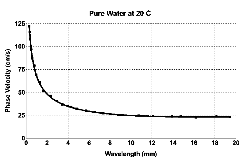
The relation $c(k)$, or equivalently $\omega (k)$, is known as the dispersion relation because it quantifies how waves of different wavenumbers that make the initial condition disperse. At any subsequent time, the shape of the interface can be reconstructed by linearly combining the translated sinusoids. These are the dynamics of small amplitude waves, specifically in this case the deep-water gravity waves. These waves are dispersive because different wavenumbers propagate at different speeds. In particular, the phase speed decreases with increasing $|k|$, as shown in Figure 13.2.

A simple dimensional argument rationalizes the propagation speed of deep-water gravity waves. For a sinusoidal wave with amplitude $h$ and wavelength $\lambda =2\pi /k$, the excess weight of the fluid above the interface and the buoyancy below the interface (wavy shaded region in Figure 13.3) scales as $({\rho }_w-{\rho }_a)g\lambda h$ per unit distance perpendicular to the plane of the page. This unbalanced force drives motion in the surrounding fluid, the motion permeates a distance of $𝒪(\lambda )$ perpendicular to the interface, decaying further away from it, as shown by the translucent region in Figure 13.3. Thus, the mass of the accelerated fluid scales as $({\rho }_a+{\rho }_w){\lambda }^2$ per unit width perpendicular to the plane of the page. The acceleration of this mass caused by the unbalanced force scales as $h/T^2$, where $T$ is the time-scale over which motion occurs, which is to be determined. Balancing this mass times the acceleration with the unbalanced force yields

$({\rho }_a+{\rho }_w){\lambda }^2\times {\displaystyle \frac{h}{T^2}}\sim ({\rho }_w-{\rho }_a)g\lambda h⟹c\propto {\displaystyle \frac{1}{T}}\sim {\left[\left({\displaystyle \frac{{\rho }_w-{\rho }_a}{{\rho }_w+{\rho }_a}}\right){\displaystyle \frac{g}{\lambda }}\right]}^{1/2}.$

(13.28)

In other words, the wave period scales inversely with ${\lambda }^{1/2}$ because the accelerated mass scales with ${\lambda }^2$ but the driving force scales proportional to $\lambda$. The dimensional dependence on the difference and sum of the density is also rationalized in this simple analysis.

In this case, we set $U=0$ for deep water gravity-capillary waves, and $g=0$ in addition for capillary waves. Repeating the analysis of §13.2.1, yields

$\omega (k)={\left[\left({\displaystyle \frac{({\rho }_w-{\rho }_a)g|k|+\sigma {|k|}^3}{{\rho }_w+{\rho }_a}}\right)\right]}^{1/2}\text{and}c(k)={\left({\displaystyle \frac{({\rho }_w-{\rho }_a){\displaystyle \frac{g}{|k|}}+\sigma |k|}{{\rho }_w+{\rho }_a}}\right)}^{1/2},$

(13.29)

for the gravity-capillary waves. In the capillary limit, these expressions become

${\omega }_{\text{cap}}(k)={\left({\displaystyle \frac{\sigma {|k|}^3}{{\rho }_w+{\rho }_a}}\right)}^{1/2}\text{and}{c}_{\text{cap}}(k)={\left({\displaystyle \frac{\sigma |k|}{{\rho }_w+{\rho }_a}}\right)}^{1/2}.$

(13.30)

A dimensional analysis interpretation of (13.30) proceeds on the same lines as the derivation of (13.28) except for the restoring force of gravity $({\rho }_w-{\rho }_a)g\lambda$ being replaced by the Laplace pressure acting over length $\lambda$, i.e. $(\sigma h/{\lambda }^2)\times \lambda$. For capillary waves, the phase speed increases with the wavenumber $|k|$, as shown in Figure 13.2.

Now we turn to some salient features of gravity-capillary waves as characterized by the dispersion relation. The expressions for the phase speeds of wave propagation for gravity, capillary, and gravity-capillary waves are plotted in Figure 13.2. The combination of gravity and capillary forces acting on the interface has complementary effect on the dispersion relation for long and short waves. On the one hand, the force of capillarity is strong for short waves, i.e. waves with short wavelength corresponding to large $k$, and therefore the gravity-capillary dispersion relation approaches that of capillary waves in the large-$k$ limit. In this regime, $c(k)$ increases with $k$. On the other hand, the gravitational restoring force dominates for long wave, i.e. waves with long wavelengths corresponding to small $k$, and the gravity-capillary dispersion relation approaches that of gravity waves in that limit. In this regime, $c(k)$ decreases with $k$. For intermediate values of $k$, the gravity-capillary phase speed has a minimum, which can be found by setting

${\displaystyle \frac{d}{d|k|}}(c{(k)}^2)={\displaystyle \frac{1}{({\rho }_w+{\rho }_a)}}\left[\sigma -{\displaystyle \frac{({\rho }_w-{\rho }_a)g}{{|k|}^2}}\right]=0⟹|k|=k_{*}={\left[{\displaystyle \frac{({\rho }_w-{\rho }_a)g}{\sigma }}\right]}^{1/2},$

(13.31)

for which

$c(k_{*})=c_{*}={\displaystyle \frac{{\left[4({\rho }_w-{\rho }_a)g\sigma \right]}^{1/4}}{{({\rho }_w+{\rho }_a)}^{1/2}}}.$

(13.32)

To get a sense of what this calculations represent, let us substitute some numbers into the expressions. The density of water ${\rho }_w={10}^3$ kg/m${}^3$ is much greater than the density of air ${\rho }_a=1.2$ kg/m${}^3$, so ${\rho }_w\pm {\rho }_a\approx {\rho }_w$. Gravity $g=9.8$ m/s${}^2$ and surface tension $\sigma =72\times {10}^{-3}$ N/m. The slowest propagating wave corresponds to wavenumber

$k_{*}={\left[{\displaystyle \frac{({\rho }_w-{\rho }_a)g}{\sigma }}\right]}^{1/2}\approx 368{\text{ m}}^{-1}.$

(13.33)

This corresponds to a wavelength of

${\lambda }_{*}={\displaystyle \frac{2\pi }{k_{*}}}=1.7\text{ cm}.$

(13.34)

Waves on the ocean surface with wavelength much larger than ${\lambda }_{*}$ are gravity waves governed by the part of the dispersion relation that approximates (13.27), whereas waves with wavelength much shorter than ${\lambda }_{*}$ are governed by (13.30) dominated by capillarity. The speed of the slowest propagating wave is

$c_{*}=23\text{ cm/s}.$

(13.35)

We shall refer to these numerical values later in this chapter.

Even though the mathematical analysis so far has been based on vanishingly small perturbation amplitude, the results of this theory apply quite well to practical situations where the amplitude of the waves is small compared to its wavelength, as shown in Figure 13.4. However, it is not merely the applicability of the analysis to the corresponding physical system that is of value, but also the fundamental concepts of wave propagation and the insight into the physical processes, which cannot be gained purely from an experimental approach. This insight ties into the subsequent analysis on instabilities and thus provides a more complete picture of the underlying physics than possible from analyses of the phenomena considered separately.

We now turn to the mechanism of overturning of the interface when the fluid above is heavier than the fluid below. The situation is analogous to balancing an inverted pendulum. While theoretically a pendulum may be balanced in an inverted configuration by having the point of support exactly below the centre of gravity of the pendulum, it is practically impossible to achieve it. The smallest, even infinitesimal, perturbation from a systematic or a random source in the environment, pushes the pendulum out of balance and the ensuing dynamics naturally pushes it further away from the equilibrium. A similar dynamics occurs when attempting to balance a semi-infinite layer of heavier fluid on top of a semi-infinite layer of lighter fluid. While the governing equations allow such a static equilibrium to exist, even an infinitesimal perturbation away from this equilibrium drives the interface away from its flat shape. The resulting fluid flow causes an overturning of the interface, causing the heavier fluid to flow downwards and pushs the lighter fluid upwards. The mechanism of this dynamics is termed as the Rayleigh-Taylor instability, after Lord Rayleigh and Geoffrey Ingram Taylor, who first presented the essential aspects of the dynamics.

A simple way to represent heavy fluid on top of light is to transform $g\to -g$ and set $U=0$ in (13.23). (Equivalently, we can switch ${\rho }_w$ and ${\rho }_a$, the only parameters that depend on the fluids.)

$({\rho }_w+{\rho }_a){\displaystyle \frac{{\partial }^{2}h}{\partial t^2}}+\left[\sigma {|k|}^3-({\rho }_w-{\rho }_a)g|k|\right]h=0.$

(13.36)

The corresponding dispersion relation

$\omega (k)={\left[\left({\displaystyle \frac{\sigma {|k|}^3-({\rho }_w-{\rho }_a)g|k|}{{\rho }_w+{\rho }_a}}\right)\right]}^{1/2}\text{and}c(k)={\left[{\displaystyle \frac{\sigma |k|-({\rho }_w-{\rho }_a){\displaystyle \frac{g}{|k|}}}{{\rho }_w+{\rho }_a}}\right]}^{1/2}.$

(13.37)

Equation (13.37) only differs from (13.29) by a negative sign, which changes the qualitative character of the dynamics. For short waves, $|k|>k_{*}$, the numerator inside the square-root for $\omega (k)$ is positive, and the wave-propagation character of the dynamics is preserved just as for gravity-capillary waves, albeit with a modified wave speed. But for long waves, , the numerator is negative and $\omega (k)$ is purely imaginary. This implies that the oscillatory behaviour of $e^{\pm i\omega t}$ in (13.25) changes to exponential growth or decay, and the wave propagation at constant speed in (13.26) changes to exponential growth or decay of sinusoids.

We will now interpret the mathematical analysis in term of its physical mechanics. According to hydrodynamic stability theory, perturbations are unavoidable in any physical system. When such a perturbation is forced on the interface, it can be decomposed into the normal modes of the system. As described in (13.26), $ϵE(k)$ and $ϵF(k)$ are the infinitesimally small amplitudes of sinusoids with wavenumber $k$ comprising the initial perturbation to the interface shape. Each of these modes evolve independently. If $\omega$ is purely imaginary, $e^{i\omega t}$ decays exponentially, so the sinusoid proportional to $F(k)$ decays exponentially, and thus its magnitude remains infinitesimal. But $e^{-i\omega t}$ grows exponentially, so the sinusoid proportional to $E(k)$ grows in magnitude, at least until the perturbation is no longer infinitesimal. Generically, perturbations forced randomly by the environment contain all normal modes of the system. Most of them are expected to decay, but if even a single mode grows exponentially, this growth continues until the flat interface shape is disrupted. The shape of the interface then more and more closely resembles the shape of the fastest growing mode. Therefore, the analysis of hydrodyanamic stability reduces to the determination of growing normal modes.

For Rayleigh-Taylor instability, the exponential growth rate is given by

$i\omega ={\left[\left({\displaystyle \frac{({\rho }_w-{\rho }_a)g|k|-\sigma {|k|}^3}{{\rho }_w+{\rho }_a}}\right)\right]}^{1/2},0\le k\le k_{*}.$

(13.38)

The growth rate is zero at $k=0$ and $k=k_{*}$, and positive in between. The growth is fastest for wavenumber given by

$|k|={\left[{\displaystyle \frac{({\rho }_w-{\rho }_a)g}{3\sigma }}\right]}^{1/2}={\displaystyle \frac{k_{*}}{\sqrt{3}}}.$

(13.39)

This is the fastest growing mode.

Physically, a depression in the interface displaces heavy fluid downwards with lighter fluid surrounding it. The lighter fluid does not provide sufficient buoyancy to compensate for the weight of the heavy fluid. Similarly, if a parcel of the lighter fluid is displaced upwards, the buoyant force on it exceeds its weight. The imbalance in both these situations continues to push the heavier fluid downward and the lighter fluid upwards. For short waves, the tension in the surface provides sufficient retoring force to overcome the driving force of gravity, but the process runs away for long waves overturning the interface. The dimensional analysis version of Rayleigh-Taylor closely parallels that of gravity-capillary waves, except gravity provides a driving force destabilizing this static flat interface instead of a restoring force. This is the physical mechanism of the Rayleigh-Taylor instability.

In this case, we restore the blowing wind and retain every variable in (13.23). The interpretation is facilitated by the substitution $({\rho }_w-{\rho }_a)g|k|+\sigma {|k|}^3=({\rho }_w+{\rho }_a)c^2{k}^2$ from (13.29), which leads to the the form of (13.23) as

${\rho }_w{\displaystyle \frac{{\partial }^{2}h}{\partial t^2}}+{\rho }_a{\left({\displaystyle \frac{\partial h}{\partial t}}+ikU\right)}^{2}h+({\rho }_w+{\rho }_a)c^2{k}^{2}h=0.$

(13.40)

The dispersion relation for this equation is the solution of

${\rho }_w{\omega }^2+{\rho }_a{(\omega +kU)}^2=({\rho }_w+{\rho }_a)c^2{k}^2.$

(13.41)

This is a quadratic equation for $\omega$, which has the solution

${\displaystyle \frac{\omega }{k}}=-{\displaystyle \frac{{\rho }_{a}U}{{\rho }_w+{\rho }_a}}\pm \sqrt{c^2-{\displaystyle \frac{U^2{\rho }_w{\rho }_a}{{({\rho }_w+{\rho }_a)}^2}}}.$

(13.42)

The variable $\omega$ is real for small $U$ if discriminant inside the square-root is positive, and sinusoids propagate at a constant speed $\omega /k$. However, for

$U>U_{\text{cr}}(k)=\left(f+f^{-1}\right)c(k),f=\sqrt{{\displaystyle \frac{{\rho }_w}{{\rho }_a}}},$

(13.43)

the discriminant is negative, $\omega$ is complex, and sinusoids grow exponentially. Here $U_{\text{cr}}(k)$ is the critical wind speed, which when exceeded perturbation to the interface with wavenumber $k$ is amplified by the wind. The smallest value for $U_{\text{cr}}$ that leads to amplification of any wavenumber occurs for $k=k_{*}$, where $c(k)$ has its minimum value of $c_{*}$. This analysis makes the following physical prediction: on a windy day as the gusts pick up, the first appearance of ripples spontaneously appearing on the interface corresponds to a wavenumber $k=k_{*}$, wavelength $\lambda ={\lambda }_{*}$ at a wind-speed

$U=U_{\text{cr}}(k_{*})=\left(f+{\displaystyle \frac{1}{f}}\right)c_{*}.$

(13.44)

For the air-water interface, using ${\rho }_a\ll {\rho }_w$, this speed is

$U\approx {\displaystyle \frac{{(4{\rho }_{w}g\sigma )}^{1/4}}{{\rho }_a^{1/2}}}=6.7\text{ m/s}.$

(13.45)

To physically understand the mechanism underlying this mathematical analysis of exponential growth, we go back to the expression for the air pressure in (13.22a) and (13.22d). Writing the air pressure in terms of interface perturbation gives

$p_a={\displaystyle \frac{{\rho }_a}{|k|}}{\left({\displaystyle \frac{\partial }{\partial t}}+ikU\right)}^{2}h.$

(13.46)

To imagine the influence of the blowing wind on a propagating wave, we substitute $h\propto a{e}^{i(kx-kct)}$ (here $c$ is the speed of propagation of the sinusoid and $a$ its amplitude) to yield the air pressure to be

$p_a\propto -{\rho }_a|k|{\left(U-c\right)}^{2}a{e}^{i(kx-kct)}.$

(13.47)

When air flows over the crests of the waves, it has the squeeze through a narrower space because of presence of the crest reduces the space available for the air to flow. This results in a speeding up when flowing over the crests, as shown in Figure 13.5. Similarly, the wind slows down when flowing through the troughs, also shown in Figure 13.5. By the Bernoulli equation, the pressure is lower where the speed is faster, i.e. the crests, and higher where the speed is slower, i.e. the troughs. This influence of the air pressure out-of-phase with the waveform acts to amplify the interface waveform and drives the instability.

It so happens that the neglect of viscosity is tolerable for the waves and the Rayleigh-Taylor instability. However, the uniform wind speed violates the no-slip condition on the interface. The presence of viscosity smoothes this profile, and the effect of this modified velocity profile needs to be accounted for in the stability analysis. This is the subject for further research for the keen student.