Chapter 11 Complex Fluids and Non-Newtonian Rheology
11.1 Constitutive laws
Up until now, we have considered Newtonian fluids with a linear relationship between the stress and rate of deformation in the fluid. For fluids consisting of small molecules, like water, this approximation works very well, even in turbulent flows with high flow rates. In realistic Newtonian flows, the separation of length and time scales mean the typical intermolecular distances or velocity distributions of individual constituents are the same whether the flow is turbulent or at rest. Hence, the energy dissipation in the fluid, which is represented by viscosity in the Newtonian constitutive law, is not affected by the flow.
When the applied flows are capable of altering the local microstructure of the fluid the classical Newtonian approximation might fail to provide an adequate mathematical model of the dynamics. For example, this is the case in solutions of colloidal particles, long flexible polymers, wormlike micelles, and similar complex fluids. These particles are significantly larger than individual molecules of typical Newtonian fluids, and the time scales of stress relaxation in these complex fluids are significantly longer than in their Newtonian counterparts. One can use the longest relaxation time to form a dimensionless group
| (11.1) |
the Weissenberg number. Here the shear rate is an invariant measure of the rate of strain in the fluid (we will talk about this more in detail below).
For small velocity gradients, , complex fluids obey the linear constitutive law, and flow like Newtonian fluids at the same Reynolds number. When the Weissenberg number is comparable to or larger than unity, complex fluids exhibit non-Newtonian behaviour and obey complicated constitutive models, often involving non-linear dependence of the local stress on the velocity gradient and the deformation history of the fluid. In this chapter we will first consider the simplest extension of a Newtonian description in which the flow only influences the instantaneous viscosity of the fluid. We will then discuss a general theory dealing with history-dependent properties of viscoelastic fluids.
11.1.1 Newtonian fluid
To begin with, let’s recap what we know for Newtonian fluids. The fluid is Newtonian if the relationship between the rate of deformation () and the stress is local, linear, instantaneous and isotropic. If the fluid is also incompressible, the Newtonian constitutive law is
| (11.2) |
where is constant and is the deviatoric stress tensor and represents the traceless () part of the stress tensor, while the pressure is the isotropic part.
11.1.2 Generalised Newtonian fluid
A generalised Newtonian fluid assumes that the applied flow only changes the energy dissipation in the fluid, represented by the viscosity, but does not change the tensorial structure of the Newtonian model. The generalised constitutive law is given by
| (11.3) |
where is the viscosity now dependent on the fluid flow. To ensure that the viscosity does not change under a coordinate transformation, which would be unphysical, the viscosity can only depend on invariants of the strain-rate tensor . The second tensorial invariant is the lowest non-trivial invariant, so we may write
| (11.4) |
Power-law fluid
For a power-law fluid the viscosity is given by
| (11.5) |
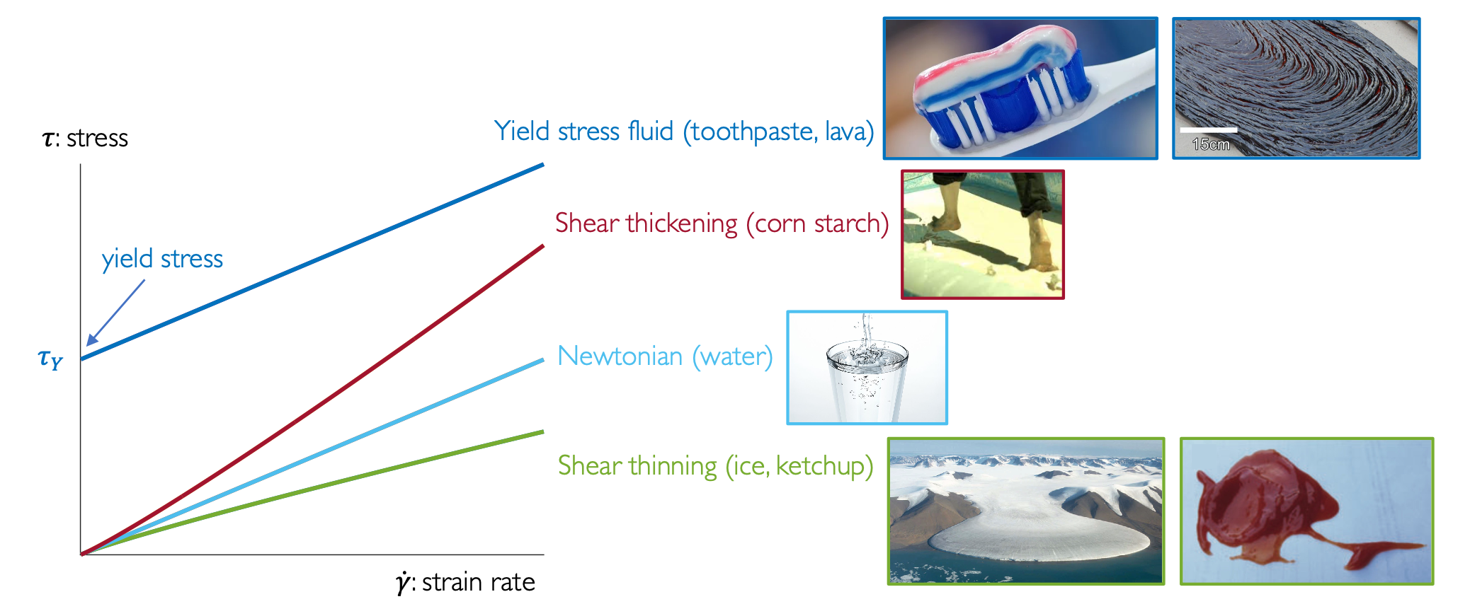
When this reduces to a Newtonian fluid. When the fluid is shear-thinning and the effective viscosity decreases with the rate of deformation; when the fluid is shear-thickening and the effective viscosity increases with the rate of deformation. Figure 11.1 gives some examples of these fluids. Note, the units of are (-pressure, -time). The constitutive law for a power-law fluid is then written as
| (11.6) |
Yield stress fluid
Yield stress fluids incorporate both solid-like and fluid like behaviour. They are characterised in terms of a yield stress . When the stress is below this yield stress there is no deformation, . When the stress is above this yield stress the fluid flows with some viscosity dependent on the strain-rate invariant.
For example, a Bingham fluid has constitutive law
| (11.7) |
and otherwise, where is a constant viscosity. Note, is the second invariant of the deviatoric stress tensor . This is chosen to decide whether the fluid is yielded or not as it does not change under a coordinate transformation and the first invariant is zero.
A Herschel-Bulkley fluid has constitutive law
| (11.8) |
and otherwise, where is the consistency with units and is the power-law index.
11.2 Poiseuille flow

As a simple example, we will consider Poiseuille flow through a two-dimensional pipe. Figure 11.2 shows the set up of a pipe with pressure gradient driving the flow at one end . is the along pipe coordinate; in the across pipe coordinate with . The velocity then satisfies the following conservation of momentum and mass equations:
| (11.9) | ||||
| (11.10) | ||||
| (11.11) |
We look for steady solutions where the flow is all in the -direction and only varies in such that . Mass conservation is automatically satisfied and the momentum equations reduce to
| (11.12) | ||||
| (11.13) |
The only non-zero component of the strain-rate tensor is , and hence . The stress components are therefore
| (11.14) |
Hence, is only a function . Since is only a function of , must also be linear in :
| (11.15) |
We have yet to consider the rheology of the fluid which we will need to do to solve for the flow field.
Newtonian fluid
For a Newtonian fluid,
| (11.16) |
Substituting this into (11.15) gives a second order ODE for subject to two boundary conditions: no-slip on the walls . Solving for the velocity we find
| (11.17) |
Power-law fluid
For a power-law fluid, we have
| (11.18) |
Substituting this into (11.15) again gives a second order ODE for subject to two boundary conditions: no-slip on the walls . We have
| (11.19) |
By symmetry, we know . Upon integrating we find velocity
| (11.20) |
Note, you need to be careful of signs here, in particular it’s useful to know that .
Bingham fluid
For a Bingham fluid, we have
| (11.21) |
The yield condition is equivalent to . Hence, we need to solve for in three different regions:
1. where . This then gives
| (11.22) |
2. where . This then gives
| (11.23) |
3. where . By matching onto the velocities either side of the unyielded region () we find plug velocity
| (11.24) |
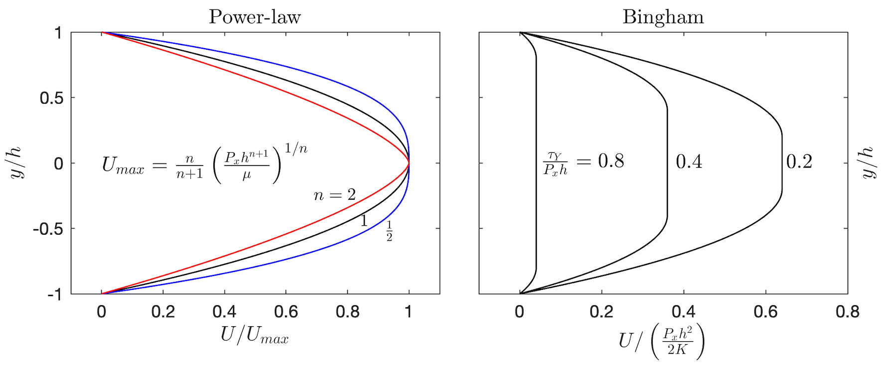
which is constant. Figure 11.3 plots the velocity profiles for Power-law and Bingham fluids. The central region is unyielded and flows in a solid plug. When the whole flow is unyielded and the plug velocity is zero i.e. the pressure gradient is not sufficient to get the flow to yield. Yield surfaces divide the unyielded and yielded parts of the flow. In this case the yield surfaces are given by .
11.3 Taylor-Couette flow

A second example is a Taylor-Couette device where we have fluid between two concentric cylinders. The inner cylinder at is fixed and the outer cylinder at rotates at a constant rotation rate , see figure 11.4. For an axisymmetric steady flow, the velocity has the form . The only non-zero strain-rate component is , and hence is the only non-zero deviatoric stress component. In cylindrical polar coordinates, the strain rate tensor and conservation of momentum in the azimuthal direction are given by
| (11.25) |
N.B. Mass conservation is automatically satisfied by the form of the assumed velocity field. This can be integrated to give stress
| (11.26) |
for some constant .
Bingham fluid
For a Bingham fluid, the constitutive law is
| (11.29) |
where because the inner cylinder is held fixed and the outer cylinder is rotating with rotation rate . Substituting this into (11.26), in the yielded region, , we have
| (11.30) |
and in the unyielded region we have
| (11.31) |
Upon integrating and applying boundary condition we find
| (11.34) |
where matching at yield surface gives relationship between the rotation rate and
| (11.35) |
Here, we have assumed that we can rotate the outer cylinder with some fixed rotation rate and cause it to yield irrespective of how large the yield stress of the Bingham fluid is. In reality, we will apply some torque to the outer cylinder and the rotation rate will depend on the magnitude of the torque, the rheology of the fluid, and the size of the cylinder. The torque on the outer cylinder is defined as
| (11.36) |
where we have used surface element . We know that on the outer cylinder , and . Hence,
| (11.37) |
Comparing this with the stress calculated above, we find a relationship between the yield surface and the magnitude of the torque
| (11.38) |
If , then we have the velocity structure as calculated above with a yield surface within the domain. If then the fluid is unyielded everywhere and performs solid body rotation. (N.B. if solid body rotation does occur everywhere then the rotation rate at the inner cylinder is also , which does not satisfy the fixed boundary condition there. Instead there must be a yielded boundary layer near the inner wall). If , the fluid is yielded everywhere.
11.4 Viscoelastic fluids
When experiments are done with polymeric fluids it is observed that the response to the shear rate is not always reproducible even if the same stress is reached. In this case, it takes time for the fluid to adjust to the flow with fluid having some memory of its flow history. A polymeric fluid will not remember its history forever, but because the molecules can be stretched by the flow it has some memory until the molecules relax. These fluids incorporate the behaviours of viscous fluids (which are instantaneous and have no memory) and elastic solids (which remember everything). Their combination gives a viscoelastic liquid that has a memory that decays with time.
11.4.1 Maxwell fluid
Let’s first look at a simple model of a viscoelastic fluid called a Maxwell fluid. Consider a shear deformation where adjacent layers of the material are shifted in the same direction along the planes relative to each other. The deformation can be described by the strain , which is approximately the total relative shift divided by the distance between the two layers assuming the displacement is small.
The shear stress for an elastic solid is given by Hooke’s law
| (11.39) |
where is the shear modulus of the material. For a Newtonian fluid the constitutive law is
| (11.40) |
where is the constant Newtonian viscosity. Graphically we could depict these two elements as a spring and a dampner. Depending on how we connect them, we form a viscoelastic fluid or viscoelastic solid.
Combined in series To combine these two relations to describe the total stress in terms of the total deformation we consider the elastic and viscous elements working in series such that the deformation is distributed () but the stress is the same (). Initially, the displacement is taken up by the spring and the dampner, but the displacement of the spring can be redistributed onto the dampner, resulting in the absence of stress at long times. Rearranging these equations we obtain
| (11.41) |
This is the constitutive law for a Maxwell fluid, which is a viscoelastic fluid.
Combined in parallel Combining these two relations in parallel, the stress is now distributed () but the deformation is the same (). In this parallel connection, unlike the previous case, the system remains under stress so long as . Rearranging these equations we obtain
| (11.42) |
This is the constitutive law for a Kelvin-Voigt solid, which is a viscoelastic solid. In this course, we will be focusing on viscoelastic fluids so we will return to the Maxwell model.
The 1D Maxwell model , where , can be solved to give
| (11.43) |
The parameter is the Maxwell relaxation time. Looking at the expression for the stress response, we see that the stress created by a stepwise deformation relaxes exponentially on a time scale (viscous-fluid-like property). Whereas, on short times and the material behaves like a solid. For example, consider the stress response to a periodic deformation with frequency , where . Substituting into the integral expression gives
| (11.44) | ||||
| (11.45) |
where are the frequency dependent viscosity and shear modulus. At short times (), and the material behaves like a solid. Whereas, at long times (), and the material behaves as a viscous fluid. The crossover between these two behaves occurs when the time scale of deformation is the same as the time scale of relaxation, .
Frame invariant? In three dimensional coordinates, the Maxwell fluid constitutive law can be written as
| (11.46) |
As we saw with the generalised Newtonian fluids above, we require the constitutive law to be frame invariant. However, the time derivative of the stress is not frame invariant. For example, if we move from a stationary lab frame to one moving with constant velocity , we have
| (11.47) |
But clearly, adding a constant velocity to the fluid should not result in any additional velocity gradients or additional stresses. Hence, the Maxwell fluid is not frame invariant. This is because the time derivatives of individual components of the stress tensor do not form a tensor themselves. To deal with this, the ordinary time derivative needs to be replaced by another derivative.
11.4.2 Oldroyd B fluid
One version of a frame invariant derivative is the upper convected derivative defined as
| (11.48) |
which transforms as a covariant tensor. N.B. there are other choices for a frame invariant derivative but we will only consider the upper convected derivative during this course. Rewriting the relationship between stress and strain-rate (11.46) using the upper convected derivative gives
| (11.49) |
to describe the polymeric stress which incorporates both viscous and elastic properties. The relaxation time of the fluid is defined as . For a polymeric fluid, there is an additional Newtonian contribution from the solvent viscosity . Hence, the total deviatoric stress tensor is written as
| (11.50) |
This model is known as the Oldroyd B model. In the limit of vanishing deformation rates it describes a Newtonian fluid with viscosity .
Oldroyd B Model:
| (11.51) | |||
| (11.52) | |||
| (11.53) | |||
| (11.54) |
where
| (11.55) |
Here, we have rewritten the Oldroyd B model in terms of variable ; a symmetric second rank tensor. This form of the model shows that tends towards its relaxed state at long times governed by long timescale at which point the polymer stress vanishes. To understand the properties of Oldroyd B fluids let’s see how it behaves in some simple fluid flows.
11.4.3 Shear flow
First consider a shear flow of the form
| (11.56) |
which only depends on () and so all variables must also only be functions of and . By construction this satisfies mass conservation. The momentum equation reduces to
| (11.57) |
where
| (11.64) |
and
| (11.71) |
Steady flow
If the strain rate is constant, the components of must also be independent of . The components then satisfy
| (11.72) | ||||
| (11.73) | ||||
| (11.74) | ||||
| (11.75) |
Hence the total stress is
| (11.78) | ||||
| (11.81) |
Compared with the Newtonian equivalent, adding polymers to the solvent causes the viscosity to increase from to , and there is now a normal stress difference
| (11.82) |
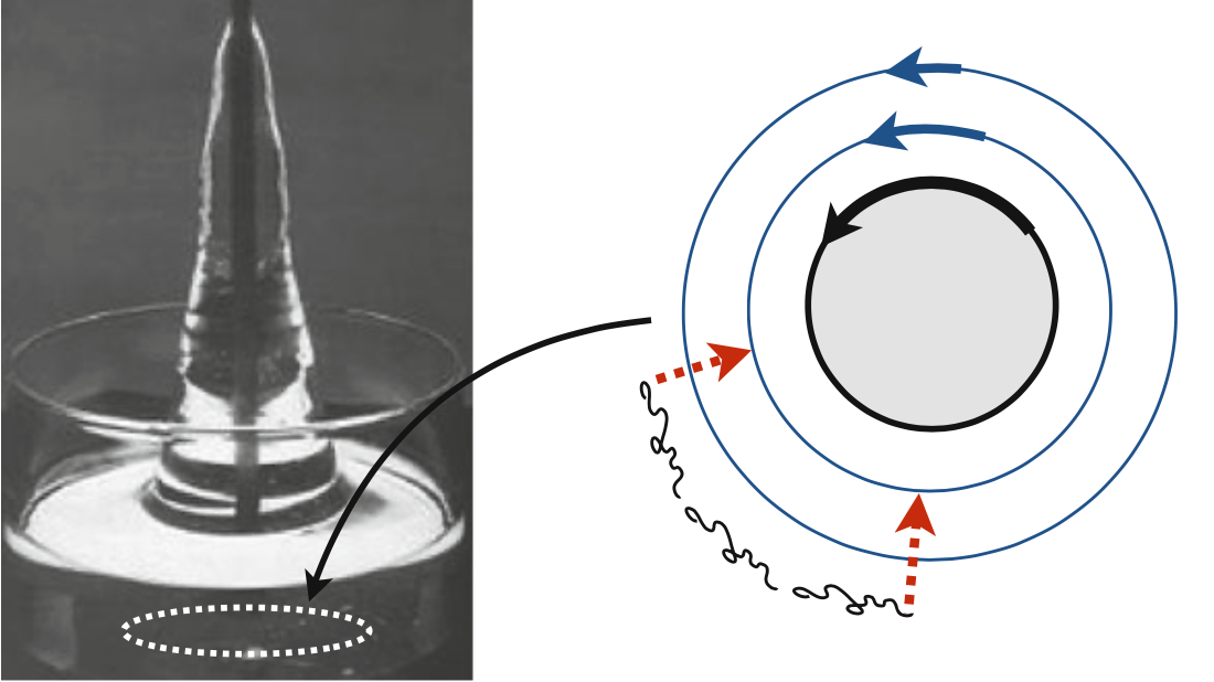
This acts in the opposite direction to pressure so is like a tension for stretched polymers along streamlines. This explains the famous rod-climbing experiments, see figure 11.5. A rod in the middle of an Oldroyd B fluid is rotated generating a shear flow in the azimuthal direction. The normal stress difference acts as a tension on the circular streamlines causing them to contract. By mass conservation, the fluid must instead move vertically, hence causing the fluid to climb up the rod.
11.4.4 Extensional flow
Now let’s consider a two dimensional extensional flow of the form
| (11.83) |
where is constant. Again, this automatically satisfies mass conservation. The strain-rate and stress tensors are
| (11.86) | ||||
| (11.93) |
with the components satisfying
| (11.100) |
Rearranging, we find
| (11.101) |
The total stress is then
| (11.104) |
where
| (11.105) |
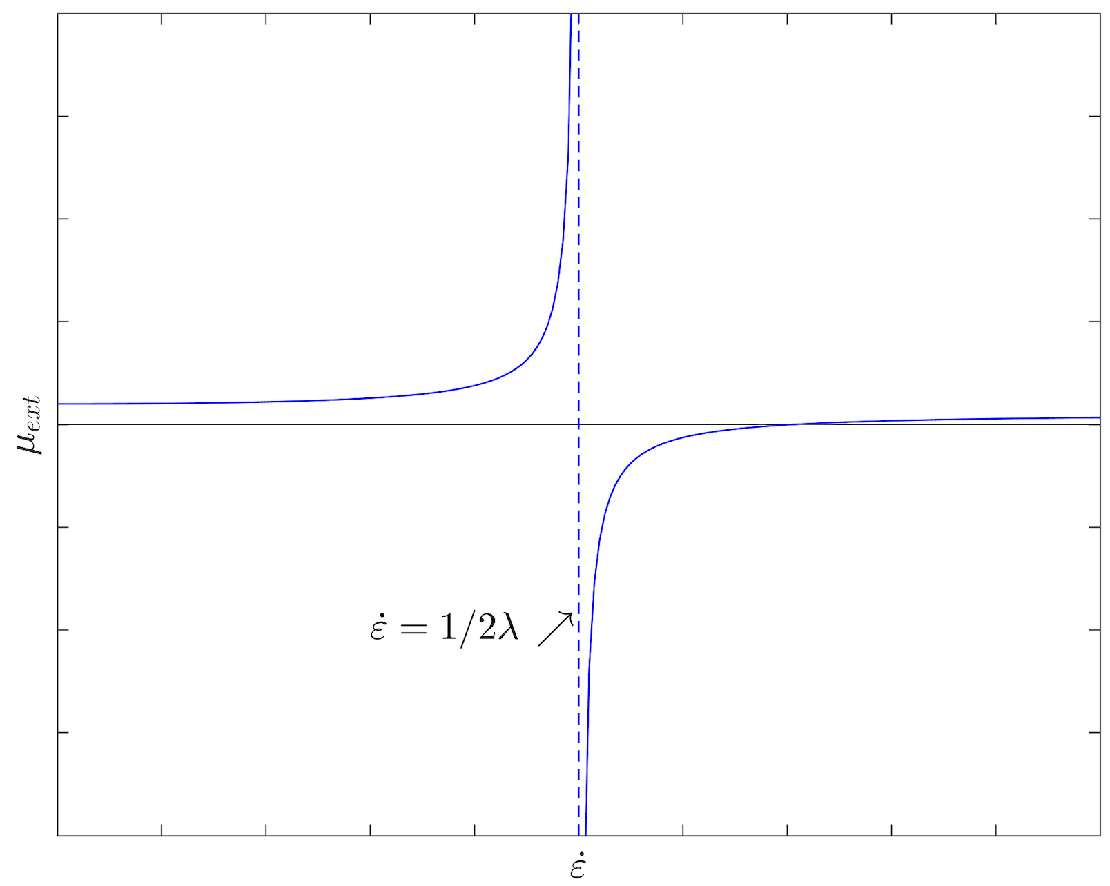
If we plot this viscosity as a function of the strain rate (figure 11.6) we see that initially the viscosity increases (hence thickens, or strain hardens). But when the viscosity diverges and then is negative for larger values. This result is clearly unphysical. This happens because the Oldroyd B model is derived using Hooke’s law which is infinitely extensible. To get around this a modification, a nonlinear spring law must be used.
11.4.5 Weakly non-linear viscoelastic fluids
A weakly non-linear flow is a situation wherein the flow changes on time scales much longer than the relaxation time, , and therefore is in some sense small and can be used as an expansion parameter. It is generally a bad practice to perform a Taylor expansion in a dimensional variable; a better expansion parameter might be , where is the typical time scale set by the flow.
From the Oldroyd B model we have
| (11.106) |
where . Let be a characteristic pressure scale, a characteristic length scale, a characteristic velocity scale. The non-dimensional version of equation (11.106) is
| (11.107) |
where . Expanding in this parameter, we may write
| (11.108) |
Substituting this into the Oldroyd B model, we recover a Newtonian constitutive law to leading order,
| (11.109) |
Putting the dimensions back in, we have
| (11.110) |
This is an example of a second-order fluid.
Second-order fluid: The simplest class of equations for viscoelastic solutions involves the expression of the stress tensor as a sum of all admissible combinations of the velocity gradient tensor. Depending on the highest algebraic power of the velocity gradient tensor involved, they are called the second-order fluid, third-order fluid, etc. For example, the deviatoric stress of the second-order fluid is given by
| (11.111) |
where are material constants.
Returning back to our Oldroyd B model, the weakly non-linear expansion is a second-order fluid with material parameters .
11.4.6 Rod climbing for a second-order fluid
For an Oldroyd B fluid we showed that there is a normal stress difference in a shear flow. In this section we will determine the steady free surface of a weakly non-linear second-order fluid caused by a rod of radius rotating at a frequency in the fluid. Flow is purely in the azimuthal direction so we write in cylindrical polars.
The flow is weakly non-linear so to leading order, the fluid behaves like a Newtonian fluid where is the only non-zero strain-rate component. In terms of the deviatoric stress components, taking to be a characteristic stress scale, and with pressure . The leading order momentum equations give
| (11.112) |
We can use these to solve for the azimuthal component of the velocity. The leading order r-momentum equation gives . The r-momentum equation at order can be used to calculate the higher order components of the stress
| (11.113) |
For the leading order balance, the fluid has a Newtonian constitutive law:
| (11.114) |
Integrating and applying boundary conditions as , gives
| (11.115) |
The vertical component of the Stokes equation gives a hydrostatic balance
| (11.116) |
We now consider the second-order contribution to the stress. Using the second-order fluid model, we have
| (11.117) |
since . Substituting into the r-momentum balance gives
| (11.118) | |||
| (11.119) |
Choosing , we arrive at
| (11.120) |
Referring back to the material parameters for the Oldroyd B model, we see the surface has height
| (11.121) |
Hence, for an Oldroyd B model, rod climbing occurs.
11.4.7 Words of caution
-
1.
The linear Maxwell model is not objective
The model is not frame invariant so none of the conclusions drawn from studying the model can be guaranteed to be physical. -
2.
Time-dependent flows in weakly non-linear viscoelastic fluids are unstable
Consider the second-order fluid model(11.122) in a two-dimensional shear flow in a channel . From momentum balance we have
(11.123) From the constitutive law, the deviatoric stress is
(11.124) These two can be combined to give
(11.125) Taking no-slip boundary conditions at the walls of a channel located at and , we write the flow velocity as a Fourier sine series:
(11.126) Substituting this into the above equation and rearranging, we find growth rates
(11.127) For polymer solutions is typically negative (recall its value based on the Oldroyd B model, ), so that is positive for sufficiently large . This implies that a steady shear flow of a second-order fluid is unstable to short-wavelength perturbations and cannot be realized. In the case of negligible inertia, achieved in the above by setting , this predicts that all Fourier modes are unstable. The implications of this result are profound: it shows that an approximation of slow flows, or, in other words, Taylor expansions of the stress in terms of the relaxation time cannot be used in time-dependent flows where any shear component would result locally in a linear instability and exponential growth of the stress. Hence, the second-order fluid and similar approximations should generally not be used to study time-dependent flows!