Chapter 12 Hydrodynamic Instability

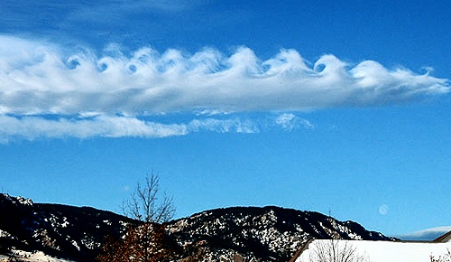
In this section we consider the Kelvin-Helmholtz instability of plane-parallel shear flow. It is this instability that is responsible for patterns observed in clouds when two air volumes move past each other with different horizontal velocities, see figure 12.1.

There are boundary conditions at the interface and at infinity. At infinity we have the perturbations decaying and the pressure tending to a constant $p_0$. Hence

${\varphi }_1,{\varphi }_2\to 0\mathrm{and}p\to p_0\mathrm{as}y\to \pm \mathrm{\infty }.$

(12.4)

At the interface we have kinematic and dynamic boundary conditions. Our kinematic boundary condition states that $y=\eta (x,t)$ remains a material surface, i.e. $D_t(\eta -y)=0$:

	${\displaystyle \frac{\partial }{\partial t}}(\eta -y)+(𝒖\cdot \mathbf{\nabla })(\eta -y)=$	$0$		(12.5)
	${\displaystyle \frac{\partial \eta }{\partial t}}+\left(U+{\displaystyle \frac{\partial \varphi }{\partial x}}\right){\displaystyle \frac{\partial \eta }{\partial x}}-{\displaystyle \frac{\partial \varphi }{\partial y}}=$	$0$		(12.6)
	${\displaystyle \frac{\partial \eta }{\partial t}}+U{\displaystyle \frac{\partial \eta }{\partial x}}-{\displaystyle \frac{\partial \varphi }{\partial y}}=$	$0\mathrm{at}y=\eta ,$		(12.7)

where we have only kept terms linear in the perturbation variables. To simplify the boundary condition further we expand about the interface $y=\eta$ using Taylor series

${{\displaystyle \frac{\partial \varphi }{\partial y}}|}_{y=\eta }={{\displaystyle \frac{\partial \varphi }{\partial y}}|}_{y=0}+{\eta {\displaystyle \frac{{\partial }^2\varphi }{\partial y^2}}|}_{y=0}+{{\displaystyle \frac{1}{2}}{\eta }^2{\displaystyle \frac{{\partial }^3\varphi }{\partial y^3}}|}_{y=0}+\mathrm{\dots }$

(12.8)

We can ignore all but the first term as the others are quadratic or higher order. The two boundary conditions are then

	${\displaystyle \frac{\partial \eta }{\partial t}}+U_1{\displaystyle \frac{\partial \eta }{\partial x}}=$	${{\displaystyle \frac{\partial {\varphi }_1}{\partial y}}|}_{y=0^{+}}$		(12.9)
	${\displaystyle \frac{\partial \eta }{\partial t}}+U_2{\displaystyle \frac{\partial \eta }{\partial x}}=$	${{\displaystyle \frac{\partial {\varphi }_2}{\partial y}}|}_{y=0^{-}}.$		(12.10)

N.B. because of the discontinuity in the base state, the perturbation to the vertical velocity $\partial \varphi /\partial y$ is not continuous at $y=0$. The dynamic boundary condition for an inviscid flow gives that the pressure must be continuous at $y=\eta$, i.e. $p_1=p_2$. To obtain the pressure at the interface we apply Bernoulli’s equation for a time-dependent irrotational flow:

$\rho {\displaystyle \frac{\partial \varphi }{\partial t}}+{\displaystyle \frac{1}{2}}\rho {|𝒖|}^2+p+\rho gy=f(t)\mathrm{at}y=\eta ,$

(12.11)

where ${|𝒖|}^2=U^2+2U\partial \varphi /\partial x+{|\mathbf{\nabla }\varphi |}^2$. After expanding about the interface $y=\eta$ using Taylor series, Bernoulli’s equation gives

${\displaystyle \frac{\partial {\varphi }_1}{\partial t}}+U_1{\displaystyle \frac{\partial {\varphi }_1}{\partial x}}={\displaystyle \frac{\partial {\varphi }_2}{\partial t}}+U_2{\displaystyle \frac{\partial {\varphi }_2}{\partial x}}.$

(12.12)

N.B. we have assumed the density of the two layers is the same, ${\rho }_1={\rho }_2=\rho$, we have taken $f(t)=\frac{1}{2}{U}_{1,2}^2+p_0$ from the far field conditions, and we have ignored the influence of gravity.

The governing equations involve $\partial /\partial x,\partial /\partial t$ and no special values of $x,t$ (unlike $\partial /\partial y$ with special value $y=0$), so we can Fourier transform in $x,t$ and look for perturbations of the form

$e^{ikx+\sigma t},$

(12.13)

with wavenumber $k$ (wavelength $2\pi /k$) and growth rate $\sigma$, which might be complex. $Re(\sigma )>0$ gives growth and $Im(\sigma )$ gives propagation. Let the interface be of the form

$\eta (x,t)=A{e}^{ikx+\sigma t},$

(12.14)

with $A$ constant, and velocity potentials

${\varphi }_1={\widehat{\varphi }}_1(y)e^{ikx+\sigma t},{\varphi }_2={\widehat{\varphi }}_2(y)e^{ikx+\sigma t}.$

(12.15)

Substituting this form into Laplace’s equation gives

${\mathbf{\nabla }}^2\varphi =0\Rightarrow -k^2\widehat{\varphi }{e}^{ikx+\sigma t}+{\displaystyle \frac{{\partial }^2\widehat{\varphi }}{\partial y^2}}{e}^{ikx+\sigma t}=0\Rightarrow \widehat{\varphi }=e^{\pm ky}.$

(12.16)

Applying boundary conditions at $\pm \mathrm{\infty }$, the velocity potentials are then

(12.17)

Using kinematic conditions (12.9-12.10) and dynamic boundary condition (12.12) we have three equations involving $A,B,C$ and $\sigma$ as a function of the wavenumber $k$:

	$(\sigma +ik{U}_1)A=$	$-kB$		(12.18)
	$(\sigma +ik{U}_2)A=$	$kC$		(12.19)
	$(\sigma +ik{U}_1)B=$	$(\sigma +ik{U}_2)C$		(12.20)
	$\Rightarrow \sigma =$	$-{\displaystyle \frac{ik(U_1+U_2)}{2}}\pm {\displaystyle \frac{k(U_1-U_2)}{2}}.$		(12.21)

Hence, the disturbance varies as

$\underset{(1)}{\underbrace{e^{ik[x-\frac{1}{2}(U_1+U_2)]}}}\underset{(2)}{\underbrace{e^{\pm \frac{k}{2}(U_1-U_2)t}}},$

(12.22)

1. 1.

   disturbance propagates at the average velocity

2. 2.

   decaying and growing mode $\Rightarrow$ flow is unstable because there is some growing disturbance

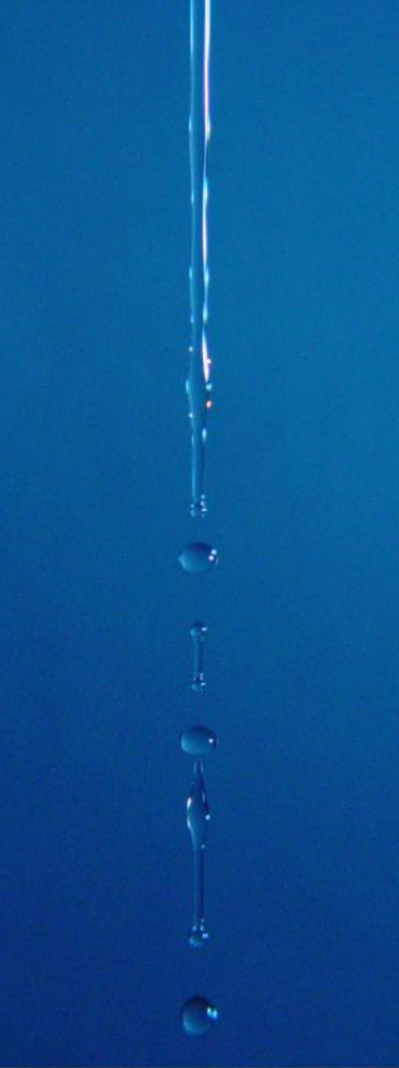
In this section we consider the Rayleigh-Plateau instability of a cylinder of inviscid fluid bounded by surface tension. It is this instability that is responsible for the break up of a water thread falling from a kitchen tap, see figure 12.3.

 A quick note on modified Bessel functions. $I_{\alpha }(x)$ and $K_{\alpha }(x)$ are the two linearly independent solutions to the modified Bessel’s equation

$x^2{\displaystyle \frac{d^{2}y}{d{x}^2}}+x{\displaystyle \frac{dy}{dx}}-(x^2+{\alpha }^2)y=0.$

(12.34)

$I_{\alpha }$ and $K_{\alpha }$ are exponentially growing and decaying functions, respectively, with properties $I_{\alpha }(x),K_{\alpha }(x)>0$ for $x>0$, $I_{\alpha }\to 0$ as $x\to 0$ for $\alpha >0$ and $K_{\alpha }\to \mathrm{\infty }$ diverges as $x\to 0$. $I_{\alpha }$ also has the property that $I_0^{\prime }(x)=I_1(x)$ and ${(x{I}_1(x))}^{\prime }=x{I}_0(x)$.  

Since we want a well-behaved solution at $r=0$ we have

${\tilde{u}}_r=A{I}_1(kr),$

(12.35)

where $A$ is a constant to be determined using boundary conditions. Using the properties of the modified Bessel functions as stated above, we can also write

$\tilde{p}=-{\displaystyle \frac{A\rho \sigma }{k}}{I}_0(kr)\mathrm{and}{\tilde{u}}_z=-{\displaystyle \frac{ik}{\rho \sigma }}\tilde{p}.$

(12.36)

We can now apply the kinematic and dynamic boundary conditions to the perturbed system. The linearised kinematic boundary condition gives

${u_r|}_{r=R_0}=R_t\Rightarrow A={\displaystyle \frac{\tilde{R}\sigma }{I_1(k{R}_0)}}.$

(12.37)

Similarily, for the linearised dynamic boundary condition

	$\widehat{𝒏}={\displaystyle \frac{\mathbf{\nabla }(r-R)}{|\mathbf{\nabla }(r-R)|}}\simeq (1,0,-ϵ\tilde{R}ik{e}^{\sigma t+ikz})\Rightarrow {\mathbf{\nabla }\cdot \widehat{𝒏}|}_{r=R_0}\simeq {\displaystyle \frac{1}{R_0}}-{\displaystyle \frac{ϵ\tilde{R}}{R_0^2}}(1-k^2{R}_0^2)e^{\sigma t+ikz}$		(12.38)
	$p_0+{ϵ\tilde{p}|}_{r=R_0}{e}^{\sigma t+ikz}=\gamma \left({\displaystyle \frac{1}{R_0}}-{\displaystyle \frac{ϵ\tilde{R}}{R_0^2}}(1-k^2{R}_0^2)e^{\sigma t+ikz}\right)\Rightarrow {\tilde{p}|}_{r=R_0}=-{\displaystyle \frac{\tilde{R}\gamma }{R_0^2}}(1-k^2{R}_0^2).$		(12.39)

Substituting in the solution for the perturbed pressure gives a dispersion relation for the growth rate $\sigma$:

${\sigma }^2={\displaystyle \frac{k\gamma }{\rho R_0^2}}{\displaystyle \frac{I_1(k{R}_0)}{I_0(k{R}_0)}}(1-k^2{R}_0^2)={\displaystyle \frac{k{R}_0\gamma }{\rho R_0^3}}{\displaystyle \frac{I_1(k{R}_0)}{I_0(k{R}_0)}}(1-k^2{R}_0^2)$

(12.40)

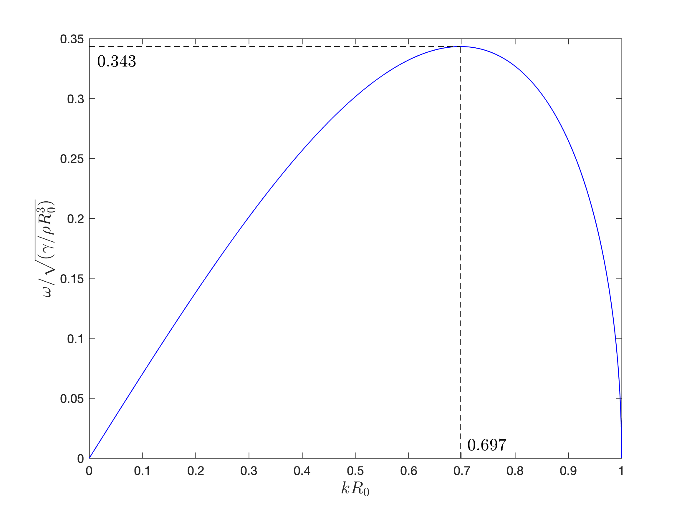
For the perturbation to grow we require the growth rate to be real (and positive). This is only the case when , since $I_1(k{R}_0),I_0(k{R}_0)>0$. Hence, the cylinder needs to be thinner than $1/k$ for the mode with wavenumber $k$ to be unstable. In other words, the cylinder is unstable to disturbances whose wavelengths exceed the circumference of the cylinder. There exists a maximum growth rate in the interval , see figure 12.3. Numerically, we find this occurs when

$k{R}_0\simeq 0.697,{\lambda }_{max}\simeq 9.02R_0,$

(12.41)

where ${\lambda }_{max}$ is the corresponding wavelength that grows most quickly. This corresponds to a timescale of breakup of

$t\sim {\displaystyle \frac{1}{{\sigma }_{max}}}\simeq 2.91\sqrt{{\displaystyle \frac{\rho R_0^3}{\gamma }}}.$

(12.42)

In this section we consider the Rayleigh instability of a cylinder of viscous fluid bounded by surface tension.

To understand when inertia can be neglected we will go through a scaling argument. To do so we will consider $k{R}_0=O(1)$ so the wavelength scales like the radius of the cylinder and there is only one length scale in the problem. Taking velocity scale $U$, lengthscale $R_0$ and timescale $1/\sigma$, we have

${\displaystyle \frac{\mu U}{R_0}}\sim p\sim {\displaystyle \frac{\gamma }{R_0}},U\sim R_0\sigma ,\sigma \sim {\displaystyle \frac{\gamma }{\mu R_0}}.$

(12.60)

Balancing terms in Navier-Stokes equations, we can neglect inertia provided

${\displaystyle \frac{\rho U}{T}}\ll {\displaystyle \frac{\mu U}{R_0^2}}\Rightarrow {\displaystyle \frac{\rho \gamma R_0}{{\mu }^2}}\ll 1.$

(12.61)

From this, we can define Ohnesorge number $Oh=\mu /\sqrt{\rho \gamma R_0}$ that relates viscous forces to inertial and surface forces. For low $Oh$ (inertial), the time scale of breakup is $t_{breakup}\sim {(\rho R_0^3/\gamma )}^{1/2}$. At high $Oh$ (viscous), the time scale of breakup is $t_{breakup}\sim \mu R_0/\gamma$.